2.1 INTRODUCTION

All the algorithms used in this project, have been designed in a way to be easily implemented in a computer based measurement instrument. This kind of systems comes to the measure through the signal processing of the input sampled data.

In this way, the computational algorithms became a fundamental part of the measurement instrument.

Generally, a main feature of a computer-based system is the presence of two fundamental parts:

1. •The hardware, which is a traditional computer, provided with a fast device for the signal processing (DSP), and which can read and store a digital input signal. The system must be able to perform measurement algorithms and some kind of data processing, in order to make a measure. Further, there must be an acquisition device for analog signals: that is, a Sample and Hold device, an Analog to Digital Converter (ADC) for having digital values from the sampled signals, and a device able to convert back the stored samples in analog signals (DAC).
   

2. •The necessary software to implement the measurement algorithms, and to run the “Virtual Instrument”.
   

Both the above points, are briefly described in the following sections, because the knowledge of the whole system is necessary to better understand the efforts and problems we faced, and the big improvement we obtain from a commercial system.

2.2 HARDWARE DESCRIPTION

The hardware we used is a personal computer (Apple Macintosh IIfx) acting as a Host Computer, provided with third party boards (National Instruments), which allow:

1. •Acquisition of electrical signal, and conversion to a sequence of digital values.
   

2. •Fast digital signal processing.
   

3. •Digital signal conversion to analog signal.
   

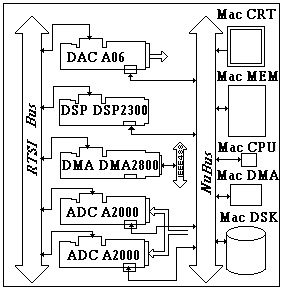
The following figure shows the third party boards placed in the host computer.

            Fig. 2.1. The logical block division of the measurement instrument hardware.

In the figure, the system bus (NuBus) is the link between prime items: on the right side there is the host computer, and on the left side the third party boards we need to complete our measurement instrument.

There is another bus just for the communication between the peripherals boards. This bus is used for control signals and is called Real Time System Integration Bus or RTSI Bus.

For the signal acquisition we used two boards (ADC A2000): each ADC board has 4 channels, so the whole system will be able to acquire up to 8 analog signals at the same time.

Of course, the maximum sampling frequency, for a single ADC board, depends on the number of channels used at the same time: 1 MHz for a single channel, 500 kHz for 2 channels, and 250 kHz for 4 channels.

Using two ADC boards, which allow sampling clock synchronisation, we double the number of channels at the same sampling frequency.

The sampled data could be stored inside the computer memory (Mac MEM), in order to be processed either by the host processor (Mac CPU) or by the digital signal processor (DSP DSP2300). It is also possible to store the data directly in the DSP memory. As we will see in the next chapters, this latter solution allows us to achieve better performances.

The DSP2300 is the board equipped with a digital signal processor, which has enough interfaces for the data transfer from and toward the other system parts.

In the system, there is more than one way to transfer data. The one used for this project is the Direct Memory Access (DMA) controller on the NB-DSP2300 board. This controller allows the system units to transfer data over the system bus: in particular, we configured it for “Block Mode” transfers. In this way, data can be transferred from the ADC buffers to the DSP Dual Port Memory (see next section). The throughput achieved is 33.7 Mbytes per second.

2.3 SIGNAL PROCESSOR ARCHITECTURE

The processor on the NB-DSP2300 board is the TI TMS320C30. This is a floating point DSP from Texas Instruments, and can reach 33.3 MFLOPS (Millions of FLOating Point instruction per Second).

The TMS320C30 is classified, from the performance, computational power, and speed point of view, in the Third Generation of Digital Signal Processors, that is in the processor class where RISC-Like (Reduced Instruction Set Computer) processor are.

The main feature is the ability of performing some phases of the instruction execution process in parallel.

This is possible because the TMS320C30 uses a mechanism known as PIPELINE. That is, there are four physical units to perform the four phases of the instruction process: FETCH, DECODE, READ, and EXECUTE. For each instruction, these phases are performed sequentially, but because there are four separate units for this task, as soon as a phase is completed for one instruction, the same unit starts again to perform the same phase on the next instruction. This mechanism allows the DSP to process in parallel up to four instructions, and therefore, to complete the instruction processing in one clock cycle, even if each single instruction needs 4 cycles to be processed.

The proper use of the pipeline is therefore a fundamental requirement if you want to achieve real time performance fast enough for the measurement process. During the coding phase of the algorithms, it is important avoid, as far as possible, the use of instructions that cause a non-sequential use of the pipeline: for instance, care must be taken for branch or jump instructions.

2.4 DSP MEMORY MAP

The DSP programming has been performed on the host computer, using LabVIEW (see next section).

It is possible to think at the DSP memory as a set of three distinct memory banks. There are two ways to access the DSP memory from the host computer: in a direct mode or through specific interrupt requests. It follows a description of the three memory banks.

1. •The first bank is a 2-kWord memory area inside the processor TMS320C30. This is the memory where to store the  real time processing procedures, because of its fast access time. We refer to this memory bank as On Chip memory, because the DSP can access it directly without any external bus.
   

2. •The second bank is a 4-kWord memory area, named Dual Ported memory. The name comes from the fact that the processor and the DMA Controller can access it simultaneously. This is the memory where to store the digital signal data. We store the data here because otherwise storing data on the host would involve specific interrupt requests with some extra-added overhead.
   

3. •The third bank is a 64-kWord memory area defined as Dual Access memory. The name comes from the fact that each on board device and each out of board device, via NuBus, can accesses it. We use this area to store the digital processing results for LabVIEW: in fact, this is the only DSP memory from where it is possible a direct data transfer to the Host Computer. This transfer can be performed through a direct addressing mechanism rather than by specific interrupts.
   

2.5 SOFTWARE ENVIRONMENT

Due to the existence of two separated processors, the one for the Host Computer and the DSP IC, the software development is performed in two separated projects and environments, depending on the target.

Concerning the host computer, the software development environment has been the LabVIEW2 tool, from National Instruments. LabVIEW represent an integrated tool, with a set of features to aid the user during the software development and the execution of applications that handle data acquisition, data storing, data processing, and processing results presentation.

The study of this kind of environment started around the beginning of the 1983: at that time, the computer based measurement instruments where programmed using traditional programming languages (such as Assembly, Basic, Fortran, C and Pascal).

The implementation of algorithms, especially the complex ones, by the use of traditional languages, was quite difficult, and causing a certain degree of complexity in reading the code itself. From here, the need of a programming tool that was able to better represent the traditional procedures used in the normal measurement instrument design, and that was, at the same time, a powerful and easy to use tool.

The definition of a new programming method, to design computer-aided measurements, has seen the introduction of the object programming in the field of the instrumentation. One of the results, it has been a new flow stream programming language, called GRAPHIC or, in short, “G”.

The G compiler used in the actual job, let the user to build several objects, named “icons”, each of them implements a well defined measurement function. These functions can be from the handling of the signal acquisition board to the measurement algorithms implementation (such as average values measurements, spectral analysis, and so on). However, the need to design “icons” as far as possible hardware independent makes the use of these existing “icons” not suitable for real time applications.

Fortunately, in LabVIEW, you have the possibility to design your custom object target dependent, and this is what we did. The purpose of those new “icons” is to handle, as fast as possible, the entire measure: from sampling until the measure results display.

Of course, the high degree of efficiency required cannot be obtained by the use of the LabVIEW G language, because such a language is not supported by any DSP compiler. Anyway, we could design new objects using a more traditional language like C.

The integration of the new C objects inside the LabVIEW environment is possible because of the features of the LabVIEW itself.

Once you have the necessary “icons”, either custom or the existing ones, you can build your final system using all the facilities provided by the “G” language.

The generic programmable “icon” is called Code Interface Node (CIN) [3]: it consists of six functions that handle variables in Pascal mode. Concerning the C language, those functions are declared as “pascal void”. It follows a brief description of three of those functions, because widely used in our project:

The function CINDispose, calls LabVIEW every time a virtual instrument with a CIN inside is removed by the memory. It is also called before the instrument compilation.

The CINInit is called during the instrument compilation, and typically reserved for variables initialisation and static memory allocation.

The CINRun is a routine where to put the user code. This routine can accept input parameters and return parameters to its output.

The compiler used has been the THINK-C for Apple Macintosh, which could be integrated within the LabVIEW environment. This compiler, for this specific usage, does not support the standard ANSI, because it must be used only for building of graphical objects: so there is no need, for instance, of the standard input and output. For these jobs, LabVIEW has already specific “icons”.

Therefore, we decided to build our projects in C language, using a reduce version of the standard C library (ANSI-small), and the library CINLib that comes with LabVIEW.

We used the modules provided by LabVIEW for all those functionalities, that do not affect the real time measurement process. For example, by the G language, we made the front panel of the measurement instrument, and we implemented the handler code to manage the communication off-line between the system units (Host Computer, DSP and acquisition boards). Always from LabVIEW, we manage the acquisition board configuration: number of channels, sampling frequency, source and trigger level, and so on. We used also the “G” language to download the DSP software (filtering, spectral analysis, and board control).

We used the modules provided by LabVIEW for all those functionalities, that do not affect the real time measurement process. For example, by the G language, we made the front panel of the measurement instrument, and we implemented the handler code to manage the communication off-line between the system units (Host Computer, DSP and acquisition boards). Always from LabVIEW, we manage the acquisition board configuration: number of channels, sampling frequency, source and trigger level, and so on. We used also the “G” language to download the DSP software (filtering, spectral analysis, and board control).

The software for the DSP has been developed in Assembly language (in order to improve the time performance of the algorithms), and compiled on the Macintosh host by the specific assembler provided by Texas Instruments, called TMS320C30 C or, for short, C30. The use of this assembler is possible only under MPW (Macintosh Programmer's Workshop) environment.

At the end, we used three languages: G and a non-standard ANSI use of THINK-C in LabVIEW for the host computer, and the Assembly C30, under MPW, for the DSP.

In order to optimise the time performance, – our main goal was to build a real time system – we divided logically and physically the processing in two parts: the part of the filter coefficients computation, for both IIR and FIR filters, and the boards status verification code, in LabVIEW; the signal processing, of course, on the DSP. We did the same also for the FFT code: the computation of trigonometric functions, coefficients for windows different from the Rectangular one, and communication and synchronisation system parameters in the host environment.

2.6 UNITS COMMUNICATION

Even if the system could be represented as a set of three parts - host, acquisition boards, and DSP - logically we need to think of it as a four layers system. We have to consider LabVIEW as a system unit by itself. In fact, it has its own virtual memory and its physical addresses cannot be retrieved directly from the host.

The approach we used for the exchange of information between the different system units, it has been the one of asynchronous communication between systems. The reasons for some of the adopted solutions were that some system units have just one bus for “talking”. Therefore, we had to avoid each kind of bus access conflict.

We had also to institute a dynamic Master-Slave hierarchy between the system units, letting the DSP to act as a Master, but only from when it starts the signal processing until the system power off. Once the DSP is started, the host can’t access anymore the DSP. Moreover, because the DSP is started from the LabVIEW, this latter one can write on the DSP memory only before starting it.

This is why, in the different instruments we made (see next chapters), LabVIEW pass parameters to the DSP by reference rather than by value; in this way, at any time the running DSP can read operating parameters directly in the host memory. While the DSP is running, LabVIEW cannot write anymore to the memory of the DSP, which is now the Master, but can modify the parameter values in its own memory. It will be up to the DSP to read or write into the LabVIEW memory.

Another optimisation it has been done for the communication between the acquisition boards and the DSP. In order to achieve the best performance in transferring the samples, the data have been compressed and sent, via DMA Controller, to blocks of the DSP memory. It is a DSP job to decompress back the data and to move it in the proper areas.

We would like to note that the whole system - Host Computer, DSP, acquisition boards, and LabVIEW – it has been sold as a system where the DSP were acting just as “mathematical coprocessor” for post processing application and not for real time ones.

With our project where the DSP is acting as Master and LabVIEW mainly as “graphical terminal support” to the DSP, the whole system has achieved new performance that the vendor itself could never expect.