Here again, the whole measurement process is performed on two distinct planes: the Host Computer and the DSP.

In LabVIEW, the first phase regards a check of the filter design specifications input by the user from the front panel (see figure 4.13).

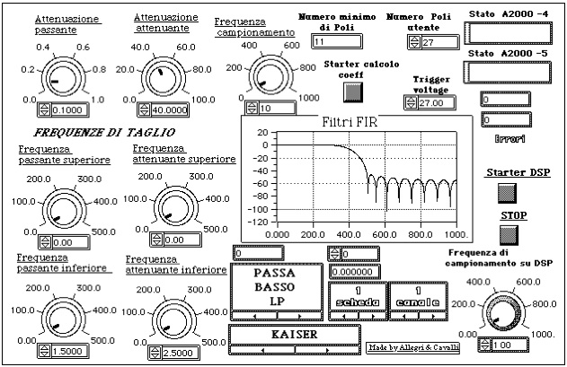
Fig 4.13 Control Panel of the measurement instrument regarding the FIR filtering process.

Once the filter specifications have been input into the system, the host program suggests automatically the minimum number of needed poles. As previously explained, this minimum number represent a precise computed constrain in case of the Kaiser window, while in all the other cases is an estimation that should be verified. In other words, for the other cases, once obtained or chose the number of poles, the user should check the Module Bode diagram (in dB). The phase diagram is not necessary in this case because the filter phases are linear.

Once all the input arguments have been properly set, the host program calculates the filter coefficients. Then resets the acquisition boards and the DSP board. Finally, download the filtering program and the filter coefficients from LabVIEW.

Filtering code and coefficients are placed into the on chip memory. The algorithm, as for the IIR filter case, performs the signal processing and, in parallel, handles the data coming from the acquisition boards. Through a mask, which depends on the channels number, the software has to unpack the sampled data coming via DMA from the acquisition boards. It places the data in the Dual Ported memory in order to perform the data processing using the software implementation of the direct structure shown in figure 4.12.

The filtered data are then placed in the Dual Access memory, ready to be transferred directly in the host memory. The use of the “end of job” or “change of parameters” flag is the same as for the IIR filters.

The following table reports the data results about the maximum sampling frequencies that allow us to perform the filtering in real time.

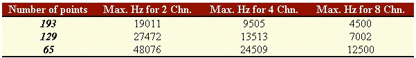
Table 4.1. Maximum frequencies in Hz to perform real time processing with all the kind of the above described windows, and for all type of filter: lowpass, highpass, bandpass, and bandstop.

The polling time for the DSP to check if there are enough input samples to be filtered is 7109ns. This time interval is necessary to guarantee that no overflow will occur in the acquisition boards. In fact, we could set other time values, but we had data overflow on the acquisition boards. The value 7109 comes after a time evaluation we did on the processing time required by the DSP. Then, this time interval has been verified run time.

Indeed, the optimal time interval depends on both the number of channels used, and on the filter poles number. In our design, we preferred to optimise the configuration where there are two channels only, and a high number of poles.

4.5 EXPERIMENTAL RESULTS

As for the IIR filter case, in this section we report some results for the FIR filters. The tests have been performed with the minimum number of poles necessary to filter the signal in real time. We required an attenuation of 0.1 dB for the pass band, and 40 dB for the rejection band. Further, we selected a sampling frequency equal to 10 kHz. The bandwidth for the transition band is 500Hz and the maximum frequency for the pass band is 1000 Hz.

Table 4.2 reports the results for a lowpass filter designed with a 53-point Kaiser window. The input signal is a sinusoid with amplitude of 4V and a variable frequency in the range from 800 to 1600 Hz.

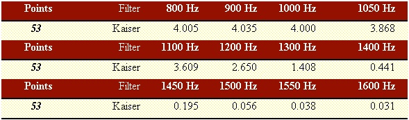
Table 4.2.

For the other filters there is no a minimum number of poles.  However, we have the estimation. With the same specifications as above described, we obtained a values equal to 45.

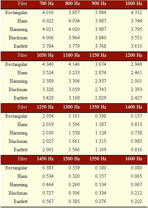
Table 4.3.

For the highpass, bandpass, and bandstop filters, we report the example of the Kaiser window.

HIGHPASS: the maximum frequency of the rejection band is 1 kHz, and the minimum of the pass band is 1500 Hz.

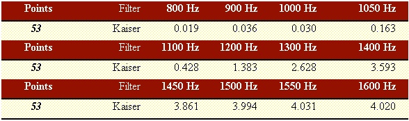
Table 4.4.

BANDPASS: the cutoff frequencies of the rejection bands are 1 kHz and 2.5 kHz. The cutoff frequencies of the pass band are 1.5 kHz and 2 kHz.

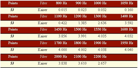
Table 4.5.

BANDSTOP: the cutoff frequencies of the pass bands are 1 kHz and 2.5 kHz. The cutoff frequencies of the rejection band are 1.5 kHz and 2 kHz.

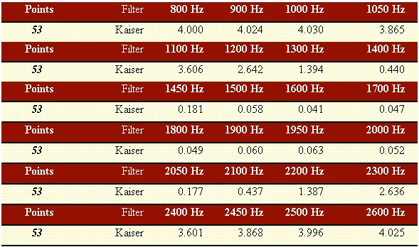
Table 4.6.

next >

< previous