5.1 INTRODUCTION

Before getting in the heart of the main feature of this project, which is an instrument for the phase spectrum analysis using specific FFT algorithms with phase error corrections, the first sections describe the conventional FFT and problems related to it. However, also a conventional FFT algorithm has been implemented in our instrument.

The FFT represents an efficient way to calculate the discrete Fourier transform (DFT) of finite time length and/or periodic data sequences.

A DFT is defined as

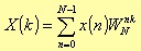
where

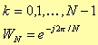
While x(n) could be a sequence of either real or complex values, typically X(k) turns out to be a sequence of complex values; N represent the number of data of the input sequence, and therefore the maximum number of harmonics the system can detect.

The calculation of the harmonics X(k) using a classical DFT leads to a high number of operations. A way to calculate the number of the required operations is the through the following steps:

1. •The product x(n)WknN is a product between two complex numbers leading to 2 additions and 4 products, which must be repeated n times with n that goes from 0 to N-1. This results in N new complex values that must be summed together. The total number of additions is 2(N-1):  N-1 for the real part, and as many for the imaginary parts.
   

2. •Therefore, for each harmonic, we have 4N products and 4(N-2) additions; this means to have 4N2 products and 4N2-2N additions for all the harmonics. If we consider N as the representative parameter for the time spent for the data processing, it is clear that as N grows, the time spent increases with quadratic law. The N2 term makes the DFT a quite heavy tool if you want to perform spectrum analyses in real time.
   

The main task of the fast Fourier transform (FFT) algorithms is to reduce as much as possible, the number of operations needed to perform the DFT.

The basic idea behind the FFT is to break up the DFT calculation of an N data sequence, in more nested DFTs over data sequences of lower sizes as the DFT level increases.

Table 5.1 shows the most common algorithms and their required number of operations [4]:

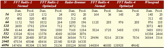
Table 5.1.

It is worth to mention, for historical reasons, the Goertzel algorithm [5], which has been the first implemented FFT algorithm: it requires about 2N2 additions and N2 multiplications. This result is not as far from the one coming from direct DFT.

An improvement can be observed with the Radix-2 algorithm where the number of operations is proportional to N log2 N, when N is a power of two. The advantages versus the Goertzel algorithm are evident as N grows.

The same principles hold for the Radix 4 and 8 [6,7], where this time N is a power of four or eight respectively.

Given a generic number of points N, there are a lot of efficient algorithms, but extremely detailed depending on prime factor decomposition of the number N.