In this section, we report the experimental results regarding the maximum frequencies that allow a real time processing.

Conventional FFT on 1024 points.

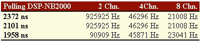
Table 6.2.

FFT with phase error correction on 1024 points.

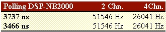
Table 6.3.

The polling information is referred to the time needed by the DSP to check if there are enough input samples to be processed. This time interval is necessary to guarantee that no overflow will occur in the acquisition boards. In fact, we could set other time values, but we had data overflow on the acquisition boards. These values come after a time estimation we did on the processing time required by the DSP. Then, these time intervals have been verified run time.

Indeed, the optimal time interval depends on both the number of channels used, and on the points number. For both the tables, in the first row there is the polling time optimised for the use of two channels. The second row is the polling time optimized for 4 channels. The third row for the 8 channels (only for the conventional FFT).

In our design, we preferred to optimise the configuration where there are two channels only, and 1024 points. About the other configurations left, we observed lower values of the maximum sampling frequencies, with differences from zero to some kHz, than the selected configuration case. In fact, the maximum sampling frequencies distribution as a function of the polling time intervals shows a flat local maximum for intervals less than the evaluated one and it decreases quicker for greater intervals than the our selected polling time. A similar behaviour has been already seen for the filters.

For instance, in the case of a polling interval equal to 3916ns (conventional FFT) the maximum frequencies are:

89685 Hz        45871 Hz        24008 Hz

for 2, 4, and 8 channels respectively.

Finally, it follows a comparison between the two FFT implementations. Generally, the phase error for the FFT with the phase error correction is of the order of 10-3 radians vs. 10-2 radians of the conventional FFT.

As for example, we consider an input periodic signal with the fundamental harmonic at 50 Hz, given by the following expression.

Let us consider an asynchronous sampling (i.e. a sampling frequency slightly different from 12800 Hz), both the FFTs on 1024 points, and a Blackman window. Moreover, the input signal is triggered on the rising edge after the zero crossing.

We can measure the following phase error on the fundamental harmonic:

2° 57’ Absolute phase error for the conventional FFT, and calculated with respect to the time origin t0.

0° 15’ Absolute phase error for the new FFT, and calculated with respect to the time t0=(N-1/2)Tc, where N is the number of the samples and Tc the sampling period [1].

Chapter 7: CONCLUSIONS

We used and transformed an existing digital measurement system, to implement a virtual instrument, able to perform measures in real time. In fact, the original system was able to perform measures only in deferred time.

Therefore, the first step has been to establish an innovative approach in the use of the existing system units, to perform real time measurements. Although the fulfilment of this project led to a use of the system at the limits, with unimaginable performance even from the system vendors, we succeed in our main goal to perform signal processing in real time. We could do that, by changing the hierarchy between the different parts forming the system. For instance, setting the DSP as the master of the communication, and the Macintosh as slave.

The sample transfer has been performed by using the DMA controller of the NB-DSP2300 board in FLYBY Block mode. This has allowed a throughput of 32MByte/second (i.e. 32 packed samples per second).

Once designed and implemented the communication between the different parts, we implemented the following measurement algorithms:

1. •IIR filtering.
   

2. •FIR IIR filtering.
   

3. •Spectral Analysis with classical FFT and related windows.
   

4. •Spectral Analysis with a new FFT with phase error correction.
   

About the IIR filtering implementation, we worked first theoretically for develop just one only and original algorithm, which was able to let us implement our desired filter.

For sure, we developed a flexible algorithm, but we were lucky to use a flexible development tools, LabVIEW. In fact, in LabVIEW each instrument can be transformed in a graphical icon to be used as a component for a new instrument.