FILTER INTRODUCTION

The digital filters have been the first application we studied and implemented in our real time measurement instrument.

Generally, a digital filter is a discrete time invariant system, implemented with a finite precision arithmetic, even if using a floating point notation.

The design of a digital filter needs three fundamental steps: the first step is to handle the system user requirements; the second step is the specification approximation through a linear time invariant discrete system, and the last step is the system implementation.

As for the analog filter design case, the system user requirements are given in the frequency domain defining a set of constrains. Unlike the analog filter design, the system user requirements are referred to the frequency characteristics of the digital signal to be filtered. When, as in our case, the signal comes from a periodic sampling and subsequently digital conversion of an analog signal, those user requirements must be bring back to the frequency requirements of the analog signal.

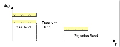
These frequency requirements come from a frequency domain subdivision in three bands (pass-band, transition-band, and rejection-band.). For each band, the user must define the limit values (it depends on the kind of filter: lowpass, highpass, bandpass, or bandstop), and their relative attenuations (in decibel), as shown in following figures (3.1 and 3.2).

Fig. 3.1. Tolerance limits and bands representation in a generic lowpass filter.


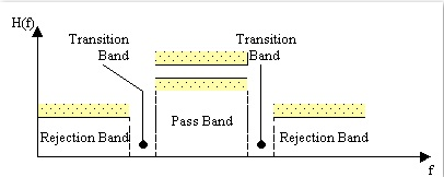
Fig. 3.2. Tolerance limits and bands representation in a generic pass band filter.

In case of a lowpass filter (figure 3.1), we need to define the following items:

 • Maximum and minimum frequencies of both the pass and rejection bands respectively (and therefore the transition bandwidth).
 • Both the pass and rejection bands attenuation.

In case of a highpass filter, we need to define the following items:

 • Minimum and maximum frequencies of both the pass and rejection bands respectively (and therefore the transition bandwidth).
 • Both the pass and rejection bands attenuation.

In case of a bandpass filter (figure 3.2), we need to define the following items:

 • The lower and the higher cut-off frequencies of the pass band.
 • The lower and the higher cut-off frequencies of the rejection bands.
 • Both the pass and rejection bands attenuation.

In case of a bandstop filter, we need to define the following items:

 • The lower and the higher cut-off frequencies of the stop band.
 • The lower and the higher cut-off frequencies of the pass bands.
 • The stop and pass band attenuations.

The problem in the filter design is to find a time invariant discrete linear system that matches the above requirements. One possible solution is to approximate the required frequency response with a rational function (case of IIR filters) or with a polynomial approximation (case of FIR filters). In both cases, the methodology used is the closed¹ form one.

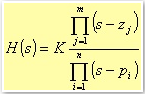
Due to the lack of literature regarding practical implementation for generic IIR filters, we developed a new methodology to compute the transfer function: the idea, deeply analysed in the next section, is to start from a generic transfer function for an analog lowpass filter with the following form

3.1

From this formula, we can come to the z-transform for all the kind of filters: lowpass, highpass, bandpass, or bandstop. The theoretic flexibility of this procedure, allows us to implement all the cases of analog filters.

---

¹ For both open and close form methodologies, see [5]

3.2 INFINITE IMPULSE RESPONSE FILTER IIR

When talking about the digital IIR filter design, the traditional way is to transform an analog filter in a digital one that matches the desired requirements. This approach is reasonable because:

 • The analog filter design technique is very advanced and well tested, so it is suitable the usage of those procedures already in use for the analog filters.
 • Most of the design methodologies for the analog filters are based on quite simple design formulae in closed form. Therefore, also these design methodologies are quite simply implemented.

In transforming an analog system in a digital one, we need to obtain the transfer function in the discrete domain (the function in thez plane) from the correlative functions of the analog filter (the function in thes plane). Typically, in this kind of transform, the general requirement is that the essential properties of the analog frequency response should be preserved in the frequency response of the resulting digital filter.

A second requirement is that if you start from a stable analog filter, you must obtain a stable digital filter. That is, the digital filter should have poles, in thez plane, only inside the unitary circle. First, this means that the imaginary axis of the s plane should be mapped in the unitary circle of the z plane, and that all the poles on the left imaginary axis of the s plane should be mapped in poles inside the unitary circle of the z plane.

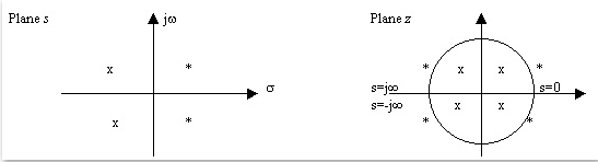
Among several design methodologies, for our system we choose the bilinear transformation method [5]. This methodology, in contrast with other methods such as the impulse invariant one, or those based on numerical resolution of the differential equations, do not show aliasing problems. In fact, the method is based on the numerical integration of the differential equation that describes the filter, and completely maps the imaginary axis of the s plane on the unitary circumference in the z plane (figure 3.3).

Fig. 3.3. Bilinear transformation where x is a pole and * is a zero.

The bilinear transformation, which is given by the following formula

3.2

converts a polynomial expression in the s domain (for instance R(s)) to one in the z domain (R(z)). Moreover, if R(s) is a rational function with a denominator degree bigger or equal than the numerator degree, the resulting function R(z) has the same numerator and denominator degrees with respect to R(s), and hence it can be implemented by a deterministic and time invariant, linear dynamic system [5].

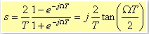
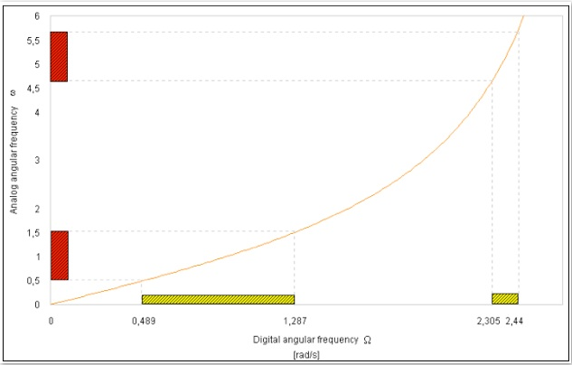
At this point, it is worth to point out, which relation exists between the frequency responses of R(s) and R(z). In particular, which is the minimum distance (the absolute value of the difference) between R(s) and R(z). Of course, the ideal case would be zero. In reality, we have a phenomenon known as frequency warping (figure 3.4):

3.3

where Ω represents the digital angular frequency and T the sampling period. This scale distortion along the digital frequency axis is:

3.4

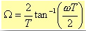
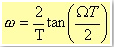
The Ω value that minimises the distance between R(s) and R(z) can be easily obtained setting

3.5

where ω is the analog angular frequency.

Fig. 3.4. How frequency warping affects amplitude responses: a yellow shaded box represents the transfer function in digital domain, while a red shaded box represents is for the analog domain. Angular frequencies are in rad/s.

As you can see from figure 3.4, you can consider as linear, only the first part at low frequencies because the curve can be approximated by a straight line. For higher frequencies there is a growing compression passing from the continuous domain to the discrete one. In fact, the range 0 ≤ ω ≤ ∞ is mapped into the range 0 ≤ ω ≤ π/2T [rad/s].

3.3 IIR FILTER PROPERTIES

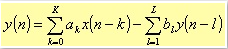
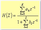
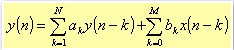
A generic IIR filter is a system that, given a set of input values x(t), generates an output y(n), such that

3.6

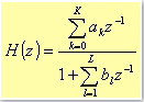
It is well known [5] that the z-transfer function for this system is

3.7

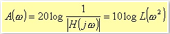
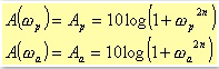
The filter attenuation, in decibel, is defined as

3.8

with

3.9

Depending on the approximation of the function L, you can obtain different filter characteristics (Butterworth, Chebyshev, and elliptical). However, the computation of the coefficients (see details in the following sections) is independent from the approximations used. In fact, the computation of the coefficients depends only on the kind of filter chosen (lowpass, highpass, bandpass, and bandstop). The transform implementing the different filters comes from the following considerations.

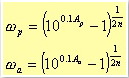
Starting from a normalised bandpass filter, it is possible to obtain a generic filter through a specific exchange of parameters. Let me consider, for instance, a normalised transfer function H_N(s) of a generic lowpass filter, and suppose the limit angular frequencies of the rejection band and the pass band are respectively ω_a and ω_p. We can define a denormalization parameter ω, such that setting

3.10

in H_N(s), if

3.11

then

3.12

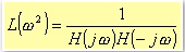
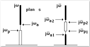
This leads to map the j axis of the s plane, into the j axis of the š plane. In particular the ranges of values [0, jω_a] and [ jω_p, ∞], is mapped respectively into the ranges [ 0, jω_p/λ] and [jω_a/λ, -∞], as shown in figure 3.5.

Fig. 3.5 Lowpass to lowpass filter transformation.

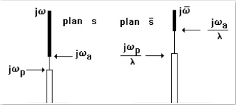
Finally, we obtain again a lowpass filter (denormalised), but with angular frequency limits given by ω_p/λ and ω_a/λ. On the other hand, to obtain a highpass filter, we need to perform the following variable change:

3.13

The new domain is shown in figure 3.6.

Fig. 3.6 Lowpass to highpass filter transformation.

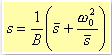
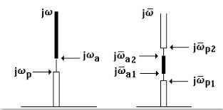
To obtain a bandpass filter from a lowpass one, you need to set

3.14

where B and ω₀ are constant (figure 3.7).

Fig. 3.7 Lowpass to bandpass filter transformation.

Last, the case of a bandstop filter from a lowpass one (figure 3.8.)

3.15

Fig. 3.8 Lowpass to bandstop filter transformation.

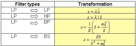
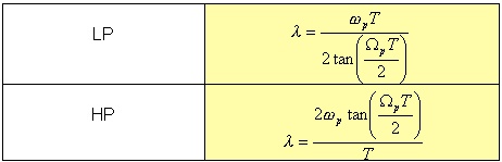
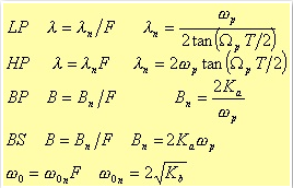
The following table summarises the four cases:

Table 3.1 Filter transformations, with a lowpass filter as a starting point.

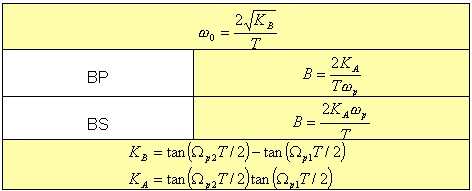
The values of the constants ω, B and ω₀ are shown in the tables 3.2 and 3.3.

Table 3.2.

Table 3.3.

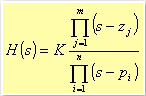
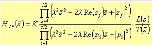
To implement the transform from H_N(s) to the not normalised transfer function H(s), we consider a generic lowpass transfer function so that we can use it for all the different IIR filter possible cases.

3.16

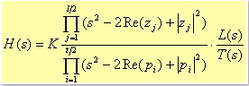
where m≤n. As the Algebra fundamental theorem states, the roots of a polynomial are complexes and conjugated two by two or real. However, our methodology needs of a transfer function with the following form

3.17

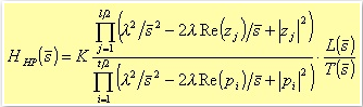
where

3.18

The form is a division of second-degree polynomial products, with a first-degree polynomial in case we have an odd number of roots. Without loss of generality, we can consider couples of complex conjugated roots plus, eventually, a real root. In fact, this real root forms the first-degree polynomial; the complex roots form the second-degree polynomial with real coefficients. For instance, even in the case of real roots, we can always refer to a second-degree polynomial, built from binomial products (which form is (s - root)), eventually plus a first-degree polynomial if we have an odd number of roots.

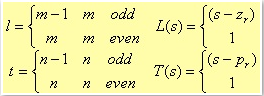
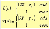
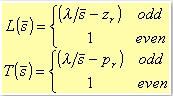
Replacing s with a function of š, shown in table 3.1, is it possible to obtain the transfer functions for the following kind of filters:

Lowpass

3.19

with

3.20

Highpass

3.21

with

3.22

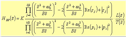
Bandpass

3.23

with

3.24

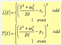
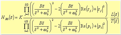
Bandstop

3.25

with

3.26

Applying the bilinear transformation

3.27

where F is the sampling frequency. Replacing š with its expression in the four different configurations, the results are the transfer functions H(z) in the z-domain:

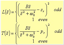
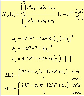
Lowpass

3.28

where z_r and p_r are the real zero and pole respectively.

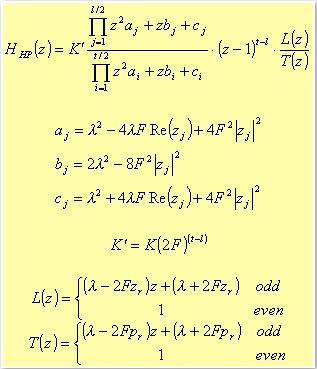
Highpass

3.29

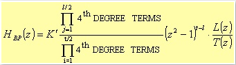
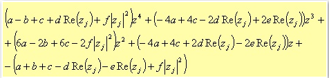
For the Bandpass case, the poles are coming from a fourth degree polynomial:

3.30

The typical expression for the fourth degree terms is

3.31

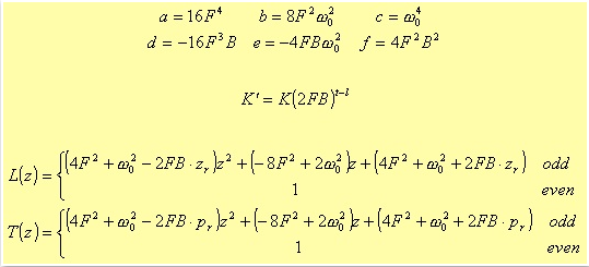
where

3.32

Bandstop

3.33

where

3.34

In this case the a, b, c, d, e, and f terms are the same as for the Bandpass filter.

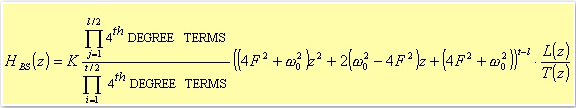
Once we have H(z) by computing the numerator and denominator products, the result is a z-transfer function in the following form

3.35

This expression allows you to implement the filter in the direct form.

We can see from tables 3.2 and 3.3 that λ, B and ω₀ are functions of the sampling frequency F=1/T. Normalising these parameters with respect to F, we obtain

3.36

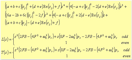
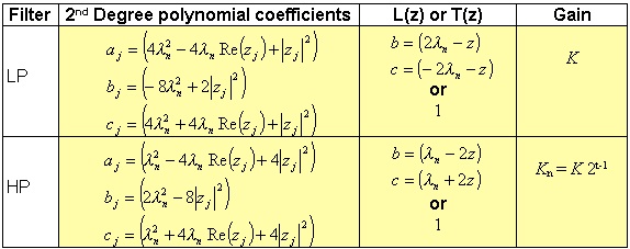
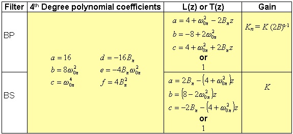
Replacing the above values into the products coefficients, the result is a new H(z) in which F does not appear anymore (Table 3.4 and 3.5). This fact avoids a possible overflow during the partial results computation of the coefficients a, b, c, d, e, and f. In fact, these coefficients depend on powers of the sampling frequency (F⁴ and F².) Hence, it's quite easy, for high sampling frequencies, to incur in overflow conditions.

Table 3.4.

Table 3.5.

At this point, it is possible to implement every kind of filter. In the following sections, we describe some of the most common filters. The filter design starts from the approximation of the attenuation function. The most simply approximation is the Butterworth one.

3.3.1 BUTTERWORTH
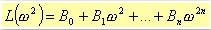
An analog filter, for instance a lowpass one with Butterworth approximation, can be designed considering the attenuation function in the following polynomial form

3.37

such that

3.38

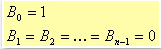
Another requirement is that the derivatives of the Taylor series L(x + h) in x=0, where x=ω², are zero for an order as higher as possible. These conditions can be obtained [2] setting

3.39

In other words, with

3.40

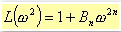
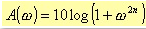
In order to have a normalised approximation, i.e. A(ω) ∼3dB at ω=1 rad/s, it is enough to set B_n=1. In this way, the attenuation is

3.41

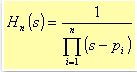
Because the roots p_i are located on the unitary radius circumference, the transfer function has the following form

3.42

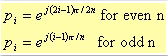
where the p_i, for i that goes from 1 to n, represent the roots of the function L(ω²) in the left half s-plane, with ω=s / j. These roots have the following form

3.43

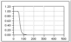
All these considerations lead to an IIR filter with Butterworth approximation, whose main characteristic is to be monotonic in both the pass and rejection bands, and with an amplitude response as flat as possible in the pass band (figure 3.9.)

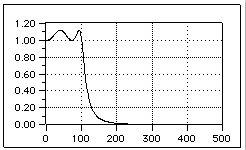
Fig. 3.9 Bode Diagram of the response module of a lowpass Butterworth filter.

For a n-order filter, increasing the n parameter, will result in a steeper filter characteristic: i.e. as n grows, the response will be close to 1 for longer in the pass band, and it will decay with a steeper slope in the rejection band. However, at the cutoff frequency, the module will be constant with a value equal to 2^-1/2.

All the 2n poles are equally distributed on half circumference whose radius is equal to the cutoff frequency on the s plane. No any pole can lie on the imaginary axes, and just one can be on the real axis, only in case n is an odd number. In this particular case the pole is located at s = -1.

If n is the order of the transfer function, for ω=ω_p or =ω_a, the attenuation is given by

3.44

That is

3.45

So setting

3.46

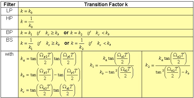
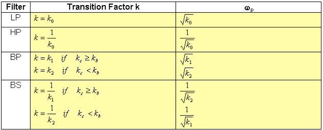
where k is given by the table 3.6, the minimum value for n to match the filter requirements is the samllest integer that satisfy the following relation

3.47

The minimum value is obtained applying the equality sign.

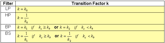
Table 3.6.

Regarding the above table, we indicated with k₀ the inverse of the transition factor k. Ω_a1 is the digital cutoff angular frequency of the first rejection band of a Bandpass filter, or the minimum angular frequency of the rejection band for a Bandstop filter.

Ω_a2 is the lower cutoff angular frequency of the second rejection band of a Bandpass filter, or the higher cutoff angular frequency of the rejection band for a Bandstop filter. Similarly, Ω_p1 and Ω_p2 are the lower and higher cut off angular frequencies, respectively, of the pass band of a Bandpass filter, and the cutoff angular frequencies of the pass bands in case of Bandstop filter.

Considering the general transfer function H(s) formulae, at the beginning of this paragraph, for a Butterworth filter we need to perform the following replacements:

3.48

3.3.2 CHEBYSHEV
If the filter requirements are given, for instance, specifying the maximum approximation error in the pass band, a better approach could be to evenly spread the precision of the approximation in the pass band, or in the rejection band, or in both the bands.

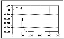
To achieve this result, you can use the Chebyshev approximation for the attenuation function L. In this way, you can obtain a constant ripple rather than a monotonic figure as for the previous filter. The filters that make use of such approximation have a frequency response module with a constant ripple behaviour in the pass band, and a monotonic behaviour in the rejection band (figure. 3.10.)

Fig. 3.10. Bode Diagram of the response module of a lowpass Chebyshev filter: with respect to the figure 3.9, here we used 3 poles instead of 6.

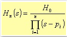
The main advantage of this type of filter, unlike the Butterworth ones, is that given the same design requirements, the filter order is lower (i.e. we need a lower n value). The normalised transfer function has the following form:

3.49

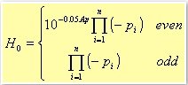
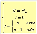
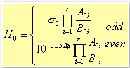
where the H₀ constant value depends on n evenness:

3.50

Once again, A_p is the pass band attenuation. In this case, the zeros of the lost function L lie on an ellipse circumscribed by the circumference of unitary radius [2].

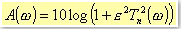
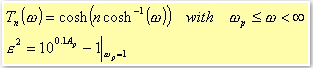
A Chebyshev filter differs from the Butterworth one, also in the way the minimum number n of poles is computed. This is due to the different expression representing the attenuation:

3.51

where

3.52

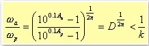
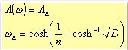
For ω=ω_a

3.53

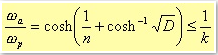
Where D, as for the Butterworth filter, is a power of the ratio ω_a/ω_p. In this way, it follows that

3.54

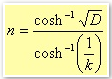
Therefore, for ω_p = 1, the minimum value for n is

3.55

Nothing is formally changed for the transition factor k, so the table 3.7 is the same as the table 3.6.

Table 3.7 Transition Factor for the Chebyshev filters: see also Table 3.6

Considering the general transfer function H(s) formulae, at the beginning of this paragraph, for a Chebyshev filter we need to perform the following replacements:

3.56

3.3.3 ELLIPTIC
The basic idea behind the elliptic filters comes considering that if you evenly spread the error over the whole pass band, as previously shown, than it is possible to match the filter design requirements with a lower filter order than when the error can grow monotonically (see Butterworth filter). Given these considerations, it is easy to think to evenly spread the error also over the rejection band. One way is the use an approximation coming from the elliptical function of Jacobi.

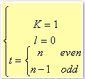
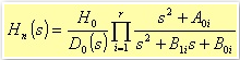
The normalised transfer function of the elliptical filter is more complex than the previous ones, and it has the following form

3.57

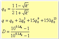
where r is (n-1)/2 when n is an odd number, and n/2 when even; D₀(s) is s + s₀ for the odd case, and 1 for the even one. Before considering the s₀ value, we need to define the following parameters:

3.58

where k is the transition factor, i.e. the ratio between the cutoff frequencies of the pass band and of the rejection one, in the case of a lowpass filter.

3.59

where A_a ed A_p are the attenuations in decibel of the rejection and pass band respectively. With these parameters, it is possible to calculate the minimum number of poles needed to match the filter design requirements.

3.60

We still need to introduce another parameter Λ

3.61

Finally

3.62

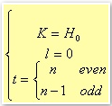
In order to represent the transfer function in more compact form, we need to define also the following parameters:

3.63

where the value of m is equal to i for odd values of n, and equal to i - 1/2 for even values of n. The variable i ranges from 1 to r.

3.64

The transfer function is then

3.65

Figure 3.11 shows the Bode diagram of the impulse response module for an elliptical filter. (The design requirements are the same as for the previous cases.)

Fig. 3.11. Bode Diagram of the response module of a lowpass elliptical filter.

Considering the general transfer function H(_s) formulae, at the beginning of this paragraph, for an elliptical filter we need to perform the following replacements:

3.66

Table 3.8 shows how to transform the design of a lowpass for the others types: highpass, bandpass, and bandstop filters.

Table 3.8

3.4 IIR Structure

There are several ways to represent time-invariant linear discrete systems using a network diagram: in fact, given a rational transfer function there are more than one network configurations.

Generally speaking, the choice between the several networks depends on the coefficients quantisation. In fact, it is well known that the error on a coefficient causes a shift of the root (pole or zero) in the complex plane, leading to a possible filter stability problem. This issue is particular important in the hardware implementations, rather than in the software ones: in our case, we use a numerical representation with 32-bit floating point, which allow us to move the problem from the design phase to the test phase [9]. Our main problem, therefore, becomes the speed performance. Hence, our best network choice is the one with the less number of operations.

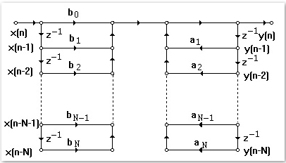
To implement the IIR filters, we adopted a direct form (see figure 3.12.). The use of this simple form will help us to achieve real time performances and to avoid big memory overheads:

3.67

Fig. 3.12. Structure to implement an IIR filter in direct form.