The implementation of deterministic systems with finite impulse response, takes the form of non-recursive algorithm. For these systems, the transfer function has the following expression:

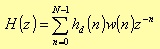
where w(n) represents the generic window.

If the impulse response is N samples long, then H(z) is a polynomial function of z -1 with a N-1 degree; that is, H(z) will have N-1 poles in z = 0, and N-1 finite zeros everywhere in the z-plane.

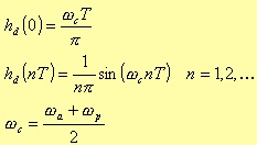
Depending on the filter type (lowpass, highpass, bandpass, and bandstop) the set of coefficients hd(n) takes1 the following form:

Lowpass

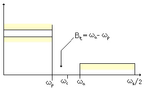
Fig. 4.1. Lowpass filter parameters in the frequency space.

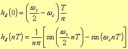
Highpass

Fig. 4.2. Highpass filter parameters in the frequency space.

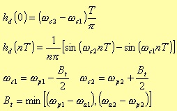
Bandpass

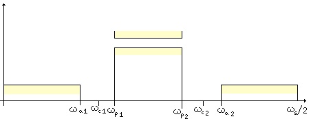
Fig. 4.3. Bandpass filter parameters in the frequency space.

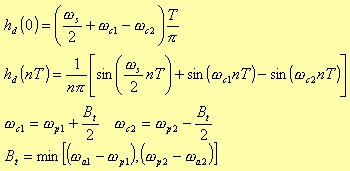
Bandstop

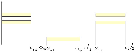
Fig. 4.4. Bandstop filter parameters in the frequency space.

To compute the coefficients we divide the different windows in three groups: Kaiser and Bartlett are considered separately, while Hann, Hamming, and Blackman are grouped together. The windows from this last group, in fact, can be obtained from a generic formula,

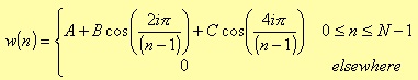
in which you should define the proper values of the constants A, B, and C depending on the specific window.

Rectangular window

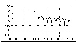
Fig. 4.5. Bode Diagram of a lowpass FIR filter with rectangular window.

Hann window

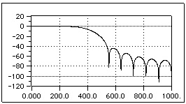
Fig. 4.6. Bode Diagram of a lowpass FIR filter with Hann window

Hamming window

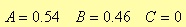
Fig. 4.7. Bode Diagram of a lowpass FIR filter with Hamming window

Blackman window

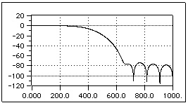
Fig. 4.8. Bode Diagram of a lowpass FIR filter with Blackman window

Bartlett window

Different is the case of the Bartlett window, which is defined as

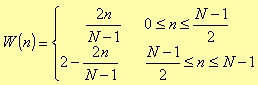
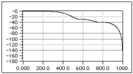
Fig. 4.9. Bode Diagram of a lowpass FIR filter with Bartlett window

For all the previous figures and for the next one, we shown the function 20log10|W(ejω)| for each window and for N = 22. It is worth pointing out that because of the symmetry of all these windows, their phase is linear. The rectangular window clearly shows a central lobe narrower than the other ones; this means that given a fixed length N, the rectangular window leads to the steepest transaction of H(ejω) at the discontinuous point of the desired impulse frequency response Hd(ejω).

Kaiser window

The last implemented window is the Kaiser window, defined as

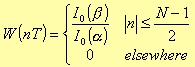
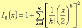
where I0 is the zero-order modified Bessel function of the first type: this function can be obtained, with the any desired degree of accuracy, using the following series with fast convergence

Further, the relation between β and α is

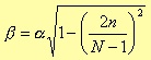
with α being an independent and empirical parameter,  which values are:

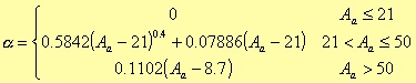
To define the Aa parameter, for instance, we have first to consider the following figure about a lowpass filter

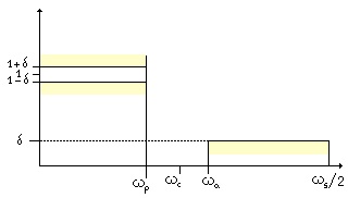
Fig. 4.10 Lowpass filter parameters in the frequency space.

If A'p and A'a denote the attenuation in decibel of the pass band and of the rejection band respectively, we could define a δ1 and a δ2 such that

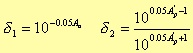
If δ represent the minimum value between δ1 and a δ2, then Aa is given by the expression

Kaiser has proved that these windows have the maximum energy in the main lobe, once the peak value for the side lobes has been defined. The  parameter could be changed in order to control the main lobe width and the height of the side lobes.

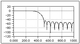
Fig. 4.11 Bode Diagram of a lowpass FIR filter with Kaiser window.

COMPUTATION OF THE NUMBER OF POLES

Different from the IIR filter where the computation of the minimum number of the poles is something well defined, here we have just an heuristic estimation based on the general dependencies of the poles number on some parameters. Generally, in fact, to guarantee the matching of the design specifications, we should have

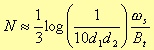
where d1 and d2 are the specific tolerances of the attenuation in the pass band and in the rejection band respectively; Bt is the transition band, while ωs is the sampling angular frequency [6].

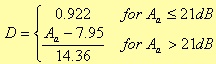
The above formula holds for all of the FIR filters, previously described, except the Kaiser windows. In the Kaiser case, we don’t have estimation, but the real minimum number of poles to guarantee the phase linearity, while matching the design specifications.

D is a parameter that depends on the rejection band attenuation.

1For instance, in the case of a lowpass filter:

next >

< previous