In the previous chapter, we saw that the use of the Radix 2 FFT requires sequences with a number of data, which is a power of two. Generally, these sequences are not symmetrical with respect to any of their terms: this means to have the errors previously described, and in particular, the phase error coming from the short-range leakage, which is the dominant error.

Fortunately, a symmetrical sequence can be obtained starting from an asymmetric one, in the following way.

Let us consider a signal s(t) sampled according to the Nyquist condition; the resulting sequence is generally not symmetric.

Once defined, however, the time origin

it is possible to consider the new sequence

such that

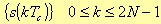
We suppose that the terms of this sequence are the samples of s(t – t0) in t0=(N-1/2)Tc within the range [-N, N-1], so now the sequence is symmetrical with respect of the point t0.

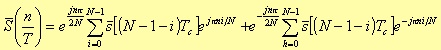
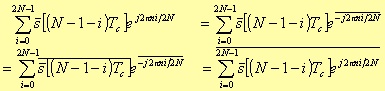
The Fourier transform of the sequence

is given by the following expression

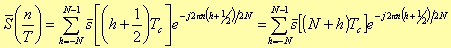
i.e.

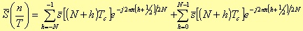
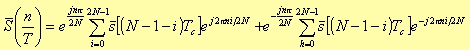
If we set i =-(h+1) in the first summation, it follows that

The two summations are not ready to be evaluated directly as FFT terms because of the exponential terms e±jπni/N instead of the terms e±j2πni/N.

The solution is to add N null points to each sum in the range N  h, i   2N-1. Obviously, the result does not change.

At this point, we have to calculate two FFT on 2N point each, with half of the points that are null data. About the input order of the signal points, using the FFT algorithm with time decimation the bit reversing is performed only on the n not null data. In fact, it is enough to alternatively place the zeros between an original point and the next one. In this way, it is also possible to considerably reduce the first computational stage of the FFT: in fact, as you can see from the figure 6.1, if x(j) = 0, the two outputs will have the same value as the input value x(i), which is not null a priori.

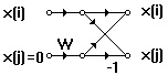
Fig. 6.1.

Therefore, instead of adding a signal of N null data, we preferred to double each input data in order to obtain an input signal as x(0), x(0), ..., x(i), x(i), .... In this way, we avoid the first computational stage of the FFT saving time (figure 6.2b). The second computational stage can be avoided too (figure 6.2c.) In fact, note that in the first memory location you store the sum between the first point and the third one, while in the third memory location you store their difference. In the second memory location there is the original point, and in the fourth one, there is the third point with opposite sign.

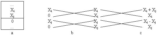
Fig. 6.2. The first three stages of the implemented FFT algorithm. a): Buffer of the generic data X with the N added zeros. We do not need a bit reversing because it is enough that the zeros come between the original data samples. b): Theoretic configuration of the input data at the first FFT stage, and c) at the second stage with the final results.

In this way, it is possible to reduce the first two FFT stages into one only stage, and to start the calculation of the FFT from the third stage.

Moreover, the fact that the original signal has positive weight factors instead of negative, as for the conventional FFT, means that is like to perform the FFT on a signal, which is out of phase for 180°.

In fact, applying the algebraic properties in the complex domain to the first summation, we have

Substituting the above expression in the original one, we have

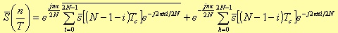
The terms inside the brackets represent two real FFT performed as there were two different signals. Figure 6.3 briefly shows the main flow diagram of the algorithm where the two summations are calculated as two FFT; the second step labeled as “Data ordering”, regards the harmonics ordering to reconstruct the spectrum of the original signal. The results from the first brackets are conjugated. Then, each data is weighted by an exponential factor. Finally, the result is the sum of the two data.

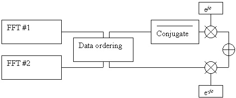
Fig. 6.3. General Flow Diagram for the FFT algorithm with phase error correction.

We obtain in this way the harmonics of the original signal, minimising the phase error.