Generally, the use of a FFT can leads to wrong results in presence of phenomena such as the aliasing or the spectrum leakage.

The former effect can be prevented by a proper use of the Shannon’s sampling theorem, and a lowpass filter for the input signal.

About the latter effect, the FFT “looks” at the signal to be analysed as if it were a periodic signal with period equal to the observation window of time. If this range of time is exactly an integer multiple of the signal period, the spectrum leakage effect does not take place.

On the contrary, there are discontinuity points at the border of the observation range with a consequent degradation of the spectral lines [1].

As for the FIR filters, for the FFT the use of proper windows can considerably reduce discontinuity at the border of the observation range, attenuating the error due to the harmonic interferences. This is the reason why we implemented with the FFT, almost the same windows (Rectangular, Hamming, Hann, Blackman, Blackman-Harris, and sin6) most of them have been already described for the FIR filters.

Moreover, we add also windows of the “Flat Top” type with 3, 4, and 5 coefficients. Their name comes from the fact that the main lobe is generally flat at the top (see figures 6.4, 6.5, and 6.6.) A typical use of these windows is to reduce the short-range leakage errors.

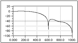
Fig. 6.4. Flat Top with 3 coefficients.

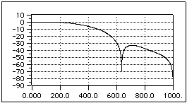
Fig. 6.5 Flat Top with 4 coefficients

Fig. 6.6 Flat Top with 5 coefficients.

The generic equation is

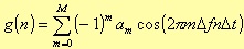
where Δfn is the frequency resolution, Δt is the time interval between two samples, and M is the significant number of spectral lines of the window. Asserting some conditions such as the coefficients normalisation

and those that regulate the asymptotic behaviour of the window

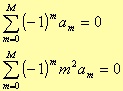
you can obtain windows with three, four, or five coefficients. In particular

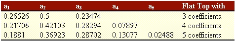
Table 6.1.