4.1 INTRODUCTION
Digital filters with finite impulse response can be considered as part of the deterministic discrete linear systems, which are invariant in time.
Their digital output, representing the samples of the filtered signal, comes from a weighted summation of a finite set of digital input data, which are the samples of the signal
to be filtered.
The coefficients of the weighted summation constitute the impulse response of the filter, and just a finite number of them are different from zero.
These filters are considered to be with finite memory;
that is, they give an output as a function of a limited number of inputs.
They are also known as non-recursive because they don't require a feedback loop in their implementation.
Although the infinite impulse response filters have very attractive properties, they also have some drawbacks.
In fact, if from on side the IIR filters generally give excellent amplitude responses, from the other side they give a phase response that is not linear.
At the contrary, the FIR filters can have phase response strictly linear.
An immediate design method for a FIR filter is to obtain an impulse response with a finite length of time by truncating an infinite impulse response.
The approximation of the design specifications of an ideal filter by truncating an ideal impulse response leads to some problems (like the Gibbs effect).
These problems can be highlighted from the study of the Fourier series convergence.
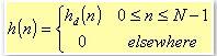
4.1
where hd(n) represents the infinite impulse response.
Generally speaking, the finite impulse response of a FIR filter can be thought as the product of the infinite impulse response with a finite length of time window.
This window, in the simple above expression, is of rectangular type.
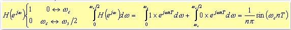
To reduce the Gibbs effects, you can truncate the Fourier series in a less abruptly way.
In other words, you can use windows different from the rectangular one.
It has been also demonstrated the main central lobe of the window Fourier transform is narrow in the frequency space.
Then, the result from the convolution between the desired frequency response and the window Fourier transform, matches quite well the design specifications.
Therefore, from one side, there is the need to have a window as short as possible in the time space (to reduce the computational complexity during the filtering processing,)
and, on the other end, we need a window as narrow as possible in the frequency space (to produce with a higher accuracy as possible, the desired response,).
Of course, these two requirements are in contrast.
Moreover, the fact of having a longer or shorter time duration of the window does not affect the amplitude of the ripples due to the Gibbs effect.
In fact, as in the case of a RECTANGULAR window (i.e. a simple abrupt truncation of the infinite impulse response,) the side lobes are not negligible.
As the window number of points grows, the main lobe peak value, as well as the ones of the side lobes, becomes bigger so that the area underneath each lobe is constant,
while the width of each lobe decreases as the number of points increase.
With this proviso, when the desired frequency response is a discontinuous function, the convolution between the desired frequency response and the window transform produces
ripples while the lobes will result overlapped in the discontinuous point.
As the number of the window points grows, the ripple amplitude does not decrease but simply grows.
It is well known from the Fourier series theory that this not uniform convergence can be reduced using a smoothly series truncation.
We can reduce the height of the secondary lobes letting the window do tend slowly to zero at its sides;
this causes the main lobe to be broaden, and therefore a less steep decay in the discontinuous point.
4.2 FILTER FIR IMPLEMENTATION
The implementation of deterministic systems with finite impulse response, takes the form of non-recursive algorithm.
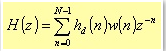
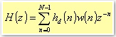
For these systems, the transfer function has the following expression:
4.2
where w(n) represents the generic window.
If the impulse response is N samples long, then H(z) is a polynomial function of z-1 with a N-1 degree; that is,
H(z) will have N-1 poles in z=0, and N-1 finite zeros everywhere in the z-plane.
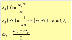
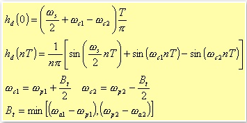
Depending on the filter type (lowpass, highpass, bandpass, and bandstop) the set of coefficients hd(n) takes1 the following form:
Lowpass
Fig. 4.1. Lowpass filter parameters in the frequency space.
4.3
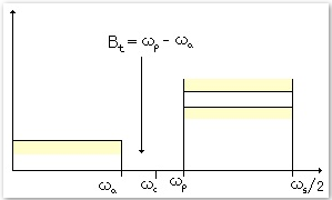
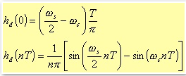
Highpass
Fig. 4.2. Highpass filter parameters in the frequency space.
4.4
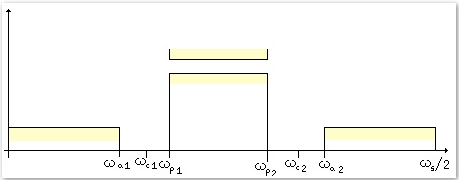
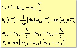
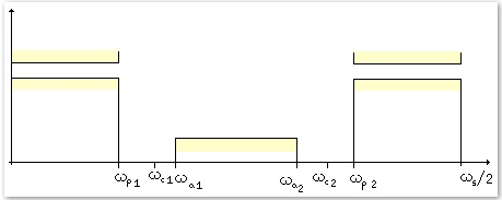
Bandpass
Fig. 4.3. Bandpass filter parameters in the frequency space.
4.5
Bandstop
Fig. 4.4. Bandstop filter parameters in the frequency space.
4.6
To compute the coefficients we divide the different windows in three groups:
Kaiser and Bartlett are considered separately, while Hann, Hamming, and Blackman are grouped together.
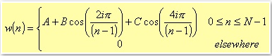
The windows from this last group, in fact, can be obtained from a generic formula,
4.7
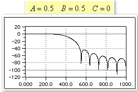
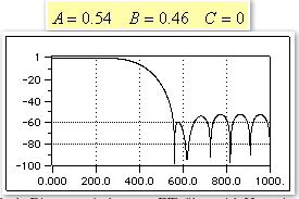
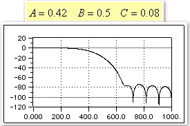
in which you should define the proper values of the constants A, B, and C depending on the specific window.
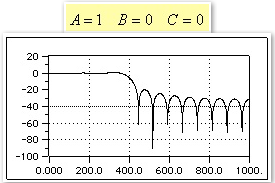
Rectangular window
Fig. 4.5. Bode Diagram of a lowpass FIR filter with rectangular window.
Hann window
Fig. 4.6. Bode Diagram of a lowpass FIR filter with Hann window.
Hamming window
Fig. 4.7. Bode Diagram of a lowpass FIR filter with Hamming window.
Blackman window
Fig. 4.8. Bode Diagram of a lowpass FIR filter with Blackman window.
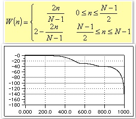
Bartlett window
Different is the case of the Bartlett window, which is defined as
Fig. 4.9. Bode Diagram of a lowpass FIR filter with Bartlett window.
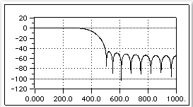
For all the previous figures and for the next one, we shown the function 20log10|W(ejω)| for each window and for N=22.
It is worth pointing out that because of the symmetry of all these windows, their phase is linear.
The rectangular window clearly shows a central lobe narrower than the other ones; this means that given a fixed length N, the rectangular window leads to the steepest transaction
of H(ejω) at the discontinuous point of the desired impulse frequency response Hd(ejω).
Kaiser window
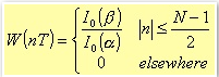
The last implemented window is the Kaiser window, defined as
4.8
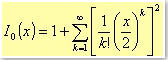
where I0 is the zero-order modified Bessel function of the first type:
this function can be obtained, with the any desired degree of accuracy, using the following series with fast convergence
4.9
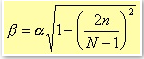
Moreover, the relation between β and α is
4.10
with α being an independent and empirical parameter, whose values are:
4.11
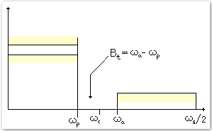
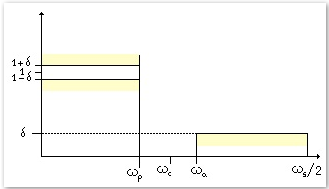
To define the Aa parameter, for instance, we have first to consider the following figure about a lowpass filter
Fig. 4.10. Lowpass filter parameters in the frequency space.
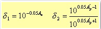
If A'p and A'a denote the attenuation in decibel of the pass band and of the rejection band respectively,
we could define a δ1 and a δ2 such that
4.12
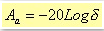
If δ represents the minimum value between δ1 and δ2, then Aa is given by the expression
4.13
Kaiser has proved that these windows have the maximum energy in the main lobe, once the peak value for the side lobes has been defined.
The parameter could be changed in order to control the main lobe width and the height of the side lobes.
Fig. 4.11. Lowpass filter parameters in the frequency space.
COMPUTATION OF THE NUMBER OF POLES
Different from the IIR filter where the computation of the minimum number of the poles is something well defined,
here we have just an heuristic estimation based on the general dependencies of the poles number on some parameters.
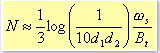
Generally, in fact, to guarantee the matching of the design specifications, we should have
4.14
where d1 and d2 are the specific tolerances of the attenuation in the pass band and in the rejection band respectively;
Bt is the transition band, while ωs is the sampling angular frequency [6].
The above formula holds for all of the FIR filters, previously described, except the Kaiser windows.
In the Kaiser case, we don't have estimation, but the real minimum number of poles to guarantee the phase linearity, while matching the design specifications.
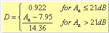
4.15
D is a parameter that depends on the rejection band attenuation.
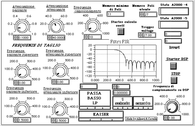
The setting of all these parameters can be done from a single front panel (see figure 3.13) in which you can also find a little display used to see the resulting filtered signal,
and the Bode diagrams for the module and the phase of the selected filter.
4.16
1For instance, in the case of a lowpass filter:
4.17
4.3 FIR Structure
As for the IIR systems, for the FIR filters there are several ways to implement the algorithms:
the Direct form, the Cascade one, and those that exploit the phase linearity1
Let us consider once again the transfer function of a generic FIR filter.
4.18
Because the all poles lie in z=0, the only elements that can be troublesome are the zeros.
Although the cascade implementation allows a better control of the zero positions, nevertheless the use of 32-bit words lets you to neglect the quantisation error,
and therefore allowing an efficient use of the Direct form.
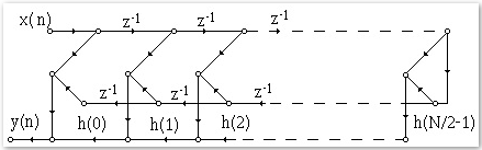
Figure 4.12 shows a Direct form structure representation.
Fig. 4.12. Implementation of a Direct form for a FIR system with an even number of points.
1The Direct form based on the exploit of the phase linearity, theoretically lets you to save half multiplications.
In practice, due to the parallelism between the multiplication and the addition operations on the DSP, we preferred to implement the normal Direct form.
4.4 INSTRUMENT IMPLEMENTATION
Here again, the whole measurement process is performed on two distinct planes: the Host Computer and the DSP.
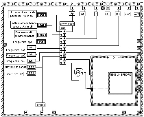
In LabVIEW, the first phase regards a check of the filter design specifications input by the user from the front panel (see figure 4.13)
Fig. 4.13. Control Panel of the measurement instrument regarding the FIR filtering process.
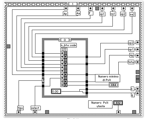
Once the filter specifications have been input into the system, the host program suggests automatically the minimum number of needed poles.
As previously explained, this minimum number represent a precise computed constrain in case of the Kaiser window, while in all the other cases is an estimation
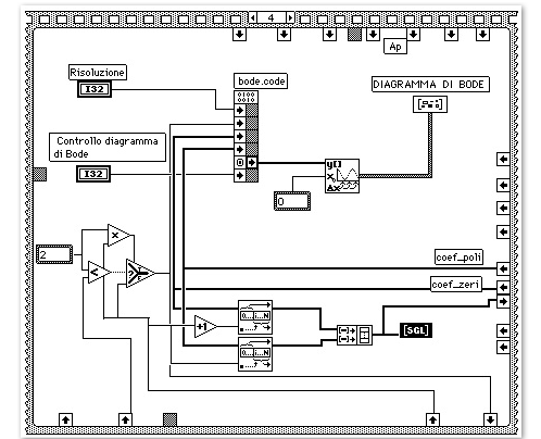
that should be verified. In other words, for the other cases, once obtained or chose the number of poles, the user should check the Module Bode diagram (in dB).
The phase diagram is not necessary in this case because the filter phases are linear.
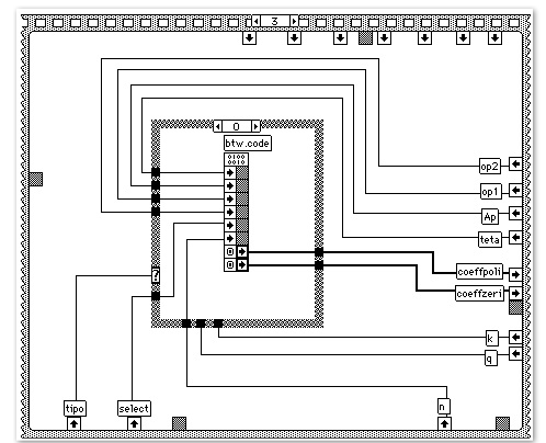
Once all the input arguments have been properly set, the host program calculates the filter coefficients.
Then resets the acquisition boards and the DSP board.
Finally, download the filtering program and the filter coefficients from LabVIEW.
Filtering code and coefficients are placed into the on chip memory.
The algorithm, as for the IIR filter case, performs the signal processing and, in parallel, handles the data coming from the acquisition boards.
Through a mask, which depends on the channels number, the software has to unpack the sampled data coming via DMA from the acquisition boards.
It places the data in the Dual Ported memory in order to perform the data processing using the software implementation of the direct structure shown in figure 4.12.
The filtered data are then placed in the Dual Access memory, ready to be transferred directly in the host memory.
The use of the end of job or change of parameters flag is the same as for the IIR filters.
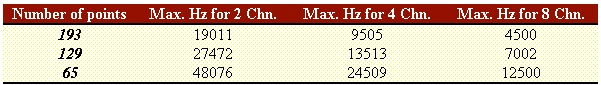
The following table reports the data results about the maximum sampling frequencies that allow us to perform the filtering in real time.
Table 4.1.Maximum frequencies in Hz to perform real time processing with all the kind of the above described windows, and for all type of filter: lowpass, highpass, bandpass, and bandstop.
The polling time for the DSP to check if there are enough input samples to be filtered is 7109ns.
This time interval is necessary to guarantee that no overflow will occur in the acquisition boards.
In fact, we could set other time values, but we had data overflow on the acquisition boards.
The value 7109 comes after a time evaluation we did on the processing time required by the DSP.
Then, this time interval has been verified run time.
Indeed, the optimal time interval depends on both the number of channels used, and on the filter poles number.
In our design, we preferred to optimise the configuration where there are two channels only, and a high number of poles.
4.5 EXPERIMENTAL RESULT
As for the IIR filter case, in this section we report some results for the FIR filters.
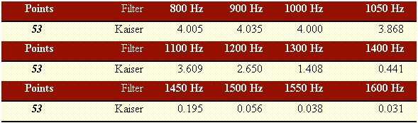
The tests have been performed with the minimum number of poles necessary to filter the signal in real time. We required an attenuation of 0.1dB for the pass band,
and 40dB for the rejection band.
Further, we selected a sampling frequency equal to 10kHz.
The bandwidth for the transition band is 500Hz and the maximum frequency for the pass band is 1000Hz.
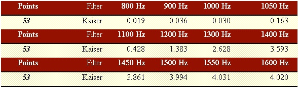
Table 4.2 reports the results for a lowpass filter designed with a 53-point Kaiser window.
The input signal is a sinusoid with amplitude of 4V and a variable frequency in the range from 800Hz to 1600Hz.
Table 4.2.
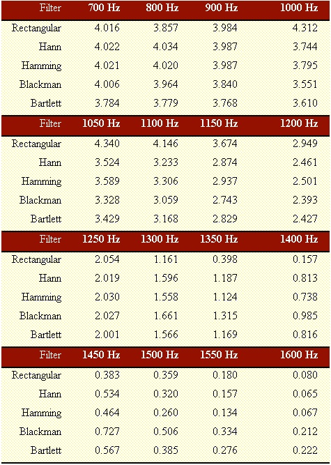
For the other filters there is no a minimum number of poles.
However, we have the estimation. With the same specifications as above described, we obtained a values equal to 45.
Table 4.3.
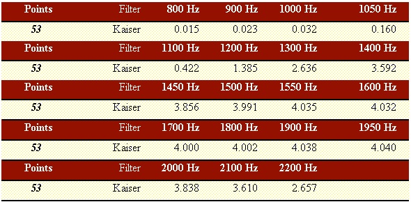
For the highpass, bandpass, and bandstop filters, we report the example of the Kaiser window.
HIGHPASS: the maximum frequency of the rejection band is 1kHz, and the minimum of the pass band is 1500Hz.
Table 4.4.
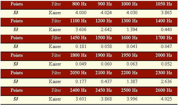
BANDPASS: the cutoff frequencies of the rejection bands are 1kHz and 2.5kHz. The cutoff frequencies of the pass band are 1.5kHz and 2kHz.
Table 4.5.
BANDSTOP: the cutoff frequencies of the pass bands are 1kHz and 2.5kHz. The cutoff frequencies of the rejection band are 1.5kHz and 2kHz.