5.1 INTRODUCTION
Before getting in the heart of the main feature of this project, which is an instrument for the phase spectrum analysis using specific FFT algorithms with phase error corrections,
the first sections describe the conventional FFT and problems related to it.
However, also a conventional FFT algorithm has been implemented in our instrument.
The FFT represents an efficient way to calculate the discrete Fourier transform (DFT) of finite time length and/or periodic data sequences.
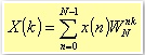
A DFT is defined as
5.1
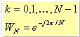
where
5.2
While x(n) could be a sequence of either real or complex values, typically X(k) turns out to be a sequence of complex values;
N represents the number of data of the input sequence, and therefore the maximum number of harmonics the system can detect.
The calculation of the harmonics X(k) using a classical DFT leads to a high number of operations.
A way to calculate the number of the required operations is the through the following steps:
• The product x(n)WknN is a product between two complex numbers leading to 2 additions and 4 products, which must be repeated
n times with n that goes from 0 to N-1.
This results in N new complex values that must be summed together.
The total number of additions is 2(N-1): N-1 for the real part, and as many for the imaginary parts.
• Therefore, for each harmonic, we have 4N products and 4(N-2) additions; this means to have 4N2 products and 4N2-2N
additions for all the harmonics. If we consider N as the representative parameter for the time spent for the data processing, it is clear that as N grows,
the time spent increases with quadratic law. The N2 term makes the DFT a quite heavy tool if you want to perform spectrum analyses in real time.
The main task of the fast Fourier transform (FFT) algorithms is to reduce as much as possible, the number of operations needed to perform the DFT.
The basic idea behind the FFT is to break up the DFT calculation of an N data sequence, in more nested DFTs over data sequences of lower sizes as the DFT level increases.
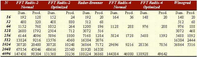
Table 5.1 shows the most common algorithms and their required number of operations [4]:
Table 5.1.
It is worth to mention, for historical reasons, the Goertzel algorithm [5], which has been the first implemented FFT algorithm:
it requires about 2N2 additions and N2 multiplications.
This result is not as far from the one coming from direct DFT.
An improvement can be observed with the Radix-2 algorithm where the number of operations is proportional to Nlog2N, when N is a power of two.
The advantages versus the Goertzel algorithm are evident as N grows.
The same principles hold for the Radix 4 and 8 [6,7], where this time N is a power of four or eight respectively.
Given a generic number of points N, there are a lot of efficient algorithms, but extremely detailed depending on prime factor decomposition of the number N.
5.2 THE OPTIMAL SOLUTION
The choice of the algorithm depends on the real time requirements and on the DSP features:
when the DSP is able to perform both a multiplication or an addition within the same CPU time, as in our case, it is not necessary to adopt the Rader Brenner solution (see table 5.1.)
In fact, in this latter case, the total number of operations is higher than the one for the optimised Radix-2 solution.
In addition, the solution proposed by Winograd [4] has been rejected mainly for two reasons:
first because the idea behind the algorithm is to reduce the number of multiplications to the detriment of the number of additions, which grows.
This could be useful in case of a typical General Purpose processor (CISC) where generally a multiplication requires more cycles than the sum.
On the contrary, looking at the table 5.1, you can see that the total number of operations (additions and products together) obtained with Winegard,
is higher than the optimised Radix-2 solution.
Second, the Winograd solution uses a recursive structure.
This leads to a different memory management not as suitable for our pipelined DSP as for a CISC machine:
the frequently function calls could prevent the CPU from a proper and efficient use of the pipeline, and the resulting code could be reach of not operation (nop) instructions.
Such situation results in a low DSP performance.
We have also rejected the Radix 4 and 8 algorithms because we chose to handle the DSP memory using blocks of 1024 word1.
The use of Radix 4 and 8 algorithms, with N=1024, let you compute FFTs only for sequences with a number of points that is only power of four or 8.
In this case, you have to implement different algorithms depending on the window width of the data to be analysed.
An attractive solution is the algorithm that considers a generic number of data, and processes the data in a packed form.
Unfortunately, also its structure is strictly dependent on the samples number, resulting in a less general and less flexible solution.
It is different the case in which the number of input data is a power of 2;
indeed, these algorithms let you to calculate the results on site, that is in the same memory location where the original input data are located without the need to move the data itself.
Somehow, also the optimised Radix 4 algorithm, as suggested by the Bellinger, is not recommended.
In fact, even if it is very efficient (about 25% more versus the Radix 2,) nevertheless it requires a considerable space of memory to store the matrices obtained from the Kronekher factorisation.
In this case, we would not be able to load these matrices in the ONCHIP memory of the DSP or even elsewhere on the DSP.
1 A word in our DSP and in the Macintosh environment is 32 bits long.
5.3 Time Decimation Radix-2 FFT
Consequently, to the above considerations, we chose to implement the optimised Radix 2 algorithm.
The adopted developing methodology is the Time Decimation.
FFT based on the time decimation have been developed breaking up the DFT calculation into smaller and smaller sub-sequences of the original input one x(n).
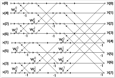
As shown in the figure 5.2, the input sequence of samples is of bit-reverse order type, while the output has a natural order.
Obviously, in this case we need a pre processing routine that takes the data from the acquisition boards and "messes up" the data order in a controlled way.
Fig. 5.2. Flow chart of time decimation FFT algorithm.
The FFT algorithm used for processing in real time the input data has been written in Assembly language.
This implemented algorithm for a real FFT, is based on the Sorensen [8] algorithm:
the N input signal points are divided, with bit-reverse order, in two main groups;
in the first group there are the points with even index, and in the second group the odd index points.
As the data enter in the butterfly structure (see figure 5.3), through a specific relation of symmetry, it is possible to calculate a priori the locations where the real data
will be placed and the so for also the complex data and their conjugates.
In this way, it is possible to avoid redundancy in the calculation, as for the conjugates values.
The number of the real data, passing through the butterfly structure, is reduced from the original N, to 2 only real data at the end of the structure:
one represents the continuous component of the input signal, at the 0 index location.
The other real value goes in the N/2 index location.
The other N-2 data left, are complex values, whose real parts go to the locations with an index that starts from 1 to N/2-1.
For the same data, the imaginary parts go to the locations with an index that starts from N-1 to N/2 +1, which is in the reverse order.
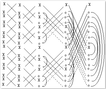
Fig. 5.3. Flow Diagram of a real Radix-2 (Sorensen) FFT. The symbol X represents the real values, while the symbol o the complex ones.
The arches show where the complex conjugate pairs are.
The hatch lines of the butterfly structure, represents where there is no need of any calculation.
Even if this algorithm needs to reorganise the data to calculate the spectrum, the amount of these operations is not as big as the number of operations required in case of an algorithm that processes a complex signal of N/2 points.
In fact, our algorithm requires exactly half multiplications and data storing instructions, and N-2 less addition of half of those required for a complex FFT.
Note that a complex FFT of a real signal always needs of a final harmonic reorganisation, anyway [7].
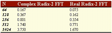
Table 5.2 reports an estimation of the time required for a complex FFT versus the results obtained with the real FFT algorithm we have implemented.
Table 5.2 Times required to process the data are in milliseconds.