3.2 INFINITE IMPULSE RESPONSE FILTER IIR

When talking about the digital IIR filter design, the traditional way is to transform an analog filter in a digital one that matches the desired requirements. This approach is reasonable because:

1. •The analog filter design technique is very advanced and well tested, so it is suitable the usage of those procedures already in use for the analog filters.
   

2. •Most of the design methodologies for the analog filters are based on quite simple design formulae in closed form. Therefore, also these design methodologies are quite simply implemented.
   

In transforming an analog system in a digital one, we need to obtain the transfer function in the discrete domain (the function in the z plane) from the correlative functions of the analog filter (the function in the s plane). Typically, in this kind of transform, the general requirement is that the essential properties of the analog frequency response should be preserved in the frequency response of the resulting digital filter.

A second requirement is that if you start from a stable analog filter, you must obtain a stable digital filter. That is, the digital filter should have poles, in the z plane, only inside the unitary circle. First, this means that the imaginary axis of the s plane should be mapped in the unitary circle of the z plane, and that all the poles on the left imaginary axis of the s plane should be mapped in poles inside the unitary circle of the z plane.

Among several design methodologies, for our system we choose the bilinear transformation method [5]. This methodology, in contrast with other methods such as the impulse invariant one, or those based on numerical resolution of the differential equations, do not show aliasing problems. In fact, the method is based on the numerical integration of the differential equation that describes the filter, and completely maps the imaginary axis of the s plane on the unitary circumference in the z plane (figure 3.3).

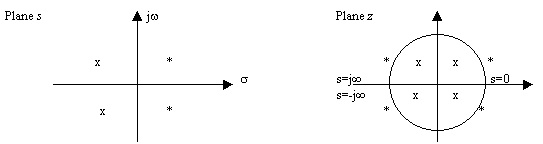
Fig. 3.3. Bilinear transformation where x is a pole and * is a zero

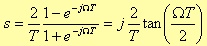
The bilinear transformation, which is given by the following formula

converts a polynomial expression in the s domain (for instance R(s)) to one in the z domain (R(z)). Moreover, if R(s) is a rational function with a denominator degree bigger or equal than the numerator degree, the resulting function R(z) has the same numerator and denominator degrees with respect to R(s), and hence it can be implemented by a deterministic and time invariant, linear dynamic system [5].

At this point, it is worth to point out, which relation exists between the frequency responses of R(s) and R(z). In particular, which is the minimum distance (the absolute value of the difference) between R(s) and R(z). Of course, the ideal case would be zero. In reality, we have a phenomenon known as “frequency warping” (figure 3.4):

where Ω represents the digital angular frequency and T the sampling period. This “scale distortion” along the digital frequency axis is:

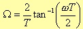
The Ω value that minimises the distance between R(s) and R(z) can be easily obtained setting

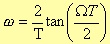
where ω is the analog angular frequency.

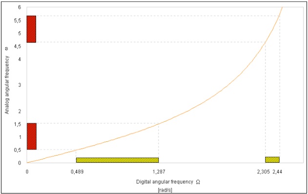
Fig. 3.4. How frequency warping affects amplitude responses: a yellow shaded box represents the transfer function in digital domain, while a red shaded box represents is for the analog domain. Angular frequencies are in rad/s.

As you can see from figure 3.4, you can consider as linear, only the first part at low frequencies because the curve can be approximated by a straight line. For higher frequencies there is a growing compression passing from the continuous domain to the discrete one. In fact, the range 0 < ω <  ∞ is mapped into the range 0 < Ω < π/2T [rad/s].

next >

< previous