3: Infinite Response Filter IIR

3.1 FILTER INTRODUCTION
The digital filters have been the first application we studied and implemented in our real time measurement instrument.
Generally, a digital filter is a discrete time invariant system, implemented with a finite precision arithmetic, even if using a floating point notation.
The design of a digital filter needs three fundamental steps: the first step is to handle the system user requirements; the second step is the specification approximation through a linear time invariant discrete system, and the last step is the system implementation.
As for the analog filter design case, the system user requirements are given in the frequency domain defining a set of constrains. Unlike the analog filter design, the system user requirements are referred to the frequency characteristics of the digital signal to be filtered. When, as in our case, the signal comes from a periodic sampling and subsequently digital conversion of an analog signal, those user requirements must be bring back to the frequency requirements of the analog signal.
These frequency requirements come from a frequency domain subdivision in three bands (pass-band, transition-band, and rejection-band.). For each band, the user must define the limit values (it depends on the kind of filter: lowpass, highpass, bandpass, or bandstop), and their relative attenuations (in decibel), as shown in following figures (3.1 and 3.2).
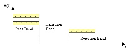
Fig. 3.1. Tolerance limits and bands representation in a generic lowpass filter
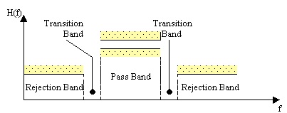
Fig. 3.2. Tolerance limits and bands representation in a generic pass band filter
In case of a lowpass filter (figure 3.1), we need to define the following items:
-
•Maximum and minimum frequencies of both the pass and rejection bands respectively (and therefore the transition bandwidth).
-
•Both the pass and rejection bands attenuation.
In case of a highpass filter, we need to define the following items:
-
•Minimum and maximum frequencies of both the pass and rejection bands respectively (and therefore the transition bandwidth).
-
•Both the pass and rejection bands attenuation.
In case of a bandpass filter (figure 3.2), we need to define the following items:
-
•The lower and the higher cut-off frequencies of the pass band.
-
•The lower and the higher cut-off frequencies of the rejection bands.
-
•Both the pass and rejection bands attenuation.
In case of a bandstop filter, we need to define the following items:
-
•The lower and the higher cut-off frequencies of the stop band.
-
•The lower and the higher cut-off frequencies of the pass bands.
-
•The stop and pass band attenuations.
The problem in the filter design is to find a time invariant discrete linear system that matches the above requirements. One possible solution is to approximate the required frequency response with a rational function (case of IIR filters) or with a polynomial approximation (case of FIR filters). In both cases, the methodology used is the closed1 form one.
Due to the lack of literature regarding practical implementation for generic IIR filters, we developed a new methodology to compute the transfer function: the idea, deeply analysed in the next section, is to start from a generic transfer function for an analog lowpass filter with the following form:
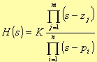
From this formula, we can come to the z-transform for all the kind of filters: lowpass, highpass, bandpass, or bandstop. The theoretic flexibility of this procedure, allows us to implement all the cases of analog filters.

1 For both open and close form methodologies, see [5]