A generic IIR filter is a system that, given a set of input values x(t), generates an output y(n), such that

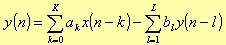
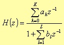
It is well known [5] that the z-transfer function for this system is

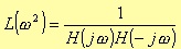
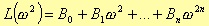
The filter attenuation, in decibel, is defined as

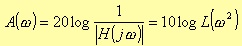
with

Depending on the approximation of the function L, you can obtain different filter characteristics (Butterworth, Chebyshev, and elliptical). However, the computation of the coefficients (see details in the following sections) is independent from the approximations used. In fact, the computation of the coefficients depends only on the kind of filter chosen (lowpass, highpass, bandpass, and bandstop). The transform implementing the different filters comes from the following considerations.

Starting from a normalised bandpass filter, it is possible to obtain a generic filter through a specific exchange of parameters. Let me consider, for instance, a normalised transfer function HN(s) of a generic lowpass filter, and suppose the limit angular frequencies of the rejection band and the pass band are respectively  ωa and ωp. We can define a “denormalization” parameter ω, such that setting

in HN(s), if

then

This leads to map the j axis of the s plane, into the j axis of the š plane. In particular the ranges of values [0, j ωa] and [ j ωp, ∞], is mapped respectively into the ranges [ 0, jωp/λ] and [jωa/λ, -∞], as shown in figure 3.5.

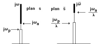
Fig. 3.5 Lowpass to lowpass filter transformation.

Finally, we obtain again a lowpass filter (denormalised), but with angular frequency limits given by ωp/λ and ωa/λ. On the other hand, to obtain a highpass filter, we need to perform the following variable change:

The new domain is shown in figure 3.6.

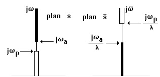
Fig. 3.6 Lowpass to highpass filter transformation.

To obtain a bandpass filter from a lowpass one, you need to set

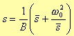
where B and ω0 are constant (figure 3.7.)

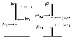
Fig. 3.7 Lowpass to bandpass filter transformation.

Last, the case of a bandstop filter from a lowpass one (figure 3.8.)

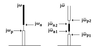
Fig. 3.8 Lowpass to bandstop filter transformation.

The following table summarises the four cases:

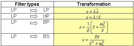
Table 3.1 Filter transformations, with a lowpass filter as a starting point.

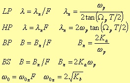
The values of the constants λ, B e ω0 is shown in the tables 3.2 and 3.3.

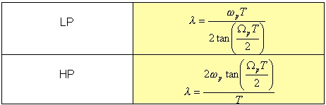
Table 3.2.

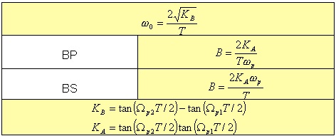
Table 3.3.

To implement the transform from HN(s) to the not normalised transfer function H(s), we consider a generic lowpass transfer function so that we can use it for all the different IIR filter possible cases.

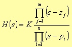
where m < n. As the Algebra fundamental theorem states, the roots of a polynomial are complexes and conjugated two by two or real. However, our methodology needs of a transfer function with the following form

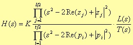
where

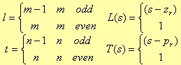
The form is a division of second-degree polynomial products, with a first-degree polynomial in case we have an odd number of roots. There won’t be any lack of generality if we consider couples of complex conjugated roots plus, eventually, a real root. In fact, this real root forms the first-degree polynomial; the complex roots form the second-degree polynomial with real coefficients. For instance, even in the case of real roots, we can always refer to a second-degree polynomial, built from binomial products (which form is (s - root)), eventually plus a first-degree polynomial if we have an odd number of roots.

Replacing s with a function of š, shown in table 3.1, you obtain the transfer functions for the following kind of filters:

Lowpass

with

Highpass

with

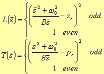
Bandpass

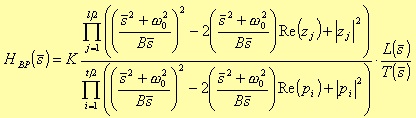
with

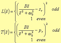
Bandstop

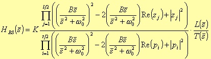
with

Applying the bilinear transformation

where F is the sampling frequency. Replacing š with its expression in the four different configurations, the result is the transfer function H(z) in the z-domain:

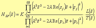
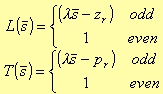
Lowpass

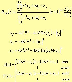
where zr and pr are the real zero and pole respectively.

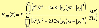
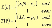
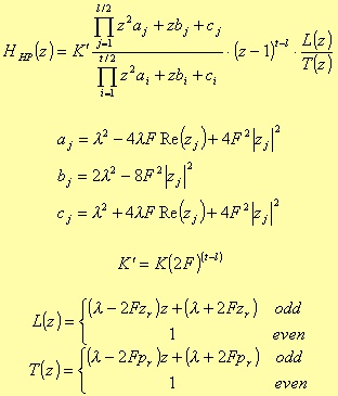
Highpass

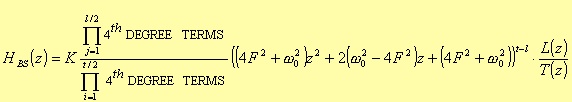
For the Bandpass case, the poles are coming from a fourth degree polynomial:

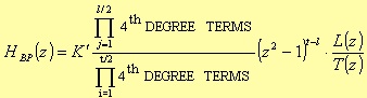
The typical expression for the fourth degree terms is

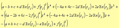
where

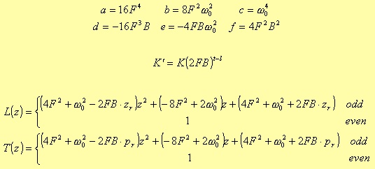
Bandstop

where

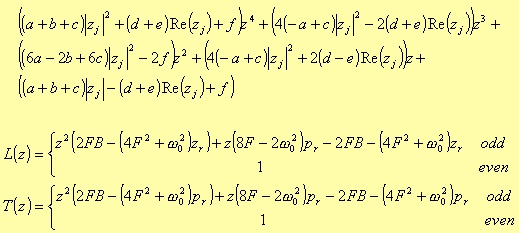
In this case the a, b, c, d, e, and f terms are the same as for the Bandpass filter.

Once you have H(z), computing the numerator and denominator products, the result is a z-transfer function in the following form

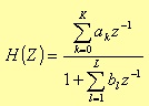
This expression allows you to implement the filter in the direct form.

As you can see from the tables 3.2 and 3.3, λ, B, and ω0 are functions of the sampling frequency F=1/T. Normalising these parameters with respect to F, you obtain

Replacing the above values into the products coefficients, the result is a new H(z) in which F does not appear anymore (Table 3.4 and 3.5). This fact avoids a possible overflow during the partial results computation of the coefficients a, b, c, d, e, and f. In fact, these coefficients depend on powers of the sampling frequency (F4 and F2 .) Hence, it’s quite easy, for high sampling frequencies, to incur in overflow conditions.

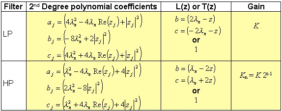
Table 3.4

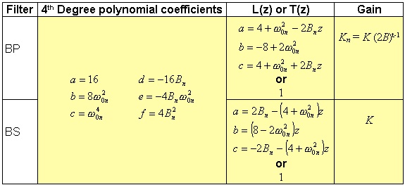
Table 3.5

At this point, it is possible to implement every kind of filter. In the following sections, we describe some of the most common filters. The filter design starts from the approximation of the attenuation function. The most simply approximation is the Butterworth one.

3.3.1 BUTTERWORTH

An analog filter, for instance a lowpass one with Butterworth approximation, can be designed considering the attenuation function in the following polynomial form

such that

Another requirement is that the derivative of the Taylor series L(x + h ), in x = 0 and where  = x2, is zero for an order as higher as possible.  These conditions can be obtained [2] setting

In other words, with

In order to have a normalised approximation, i.e. A(ω) ~3dB at ω=1 rad/s, it is enough to set Bn = 1. In this way, the attenuation is

Because the roots pi are located on the unitary radius circumference, the transfer function has the following form

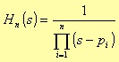
where the pi, for i that goes from 1 to n, represent the roots of the function L(ω2) in the left half s-plane, with  ω= s/j. These roots have the following form

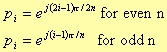
All these considerations lead to an IIR filter with Butterworth approximation, whose main characteristic is to be monotonic in both the pass and rejection bands, and with an amplitude response as flat as possible in the pass band (figure 3.9.)

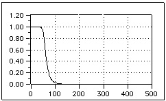
  Fig. 3.9. Bode Diagram of the response module of a lowpass Butterworth filter.

For a n-order filter, increasing the n parameter, will result in a steeper filter characteristic: i.e. as n grows, the response will be close to 1 for longer in the pass band, and it will decay with a steeper slope in the rejection band. However, at the cutoff frequency, the module will be constant with a value equal to 2-1/2.

All the 2n poles are equally distributed on half circumference whose radius is equal to the cutoff frequency on the s plane. No any pole can lie on the imaginary axes, and just one can be on the real axis, only in case n is an odd number. In this particular case the pole is located at s = -1.

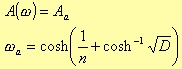
If n is the order of the transfer function, for  ω= ωp or = ωa, the attenuation is given by

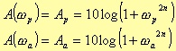
That is

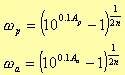
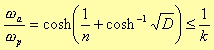
So setting

where k is given by the table 3.6. The values for n to match the filter requirements are

The minimum value is obtained applying the equality sign.

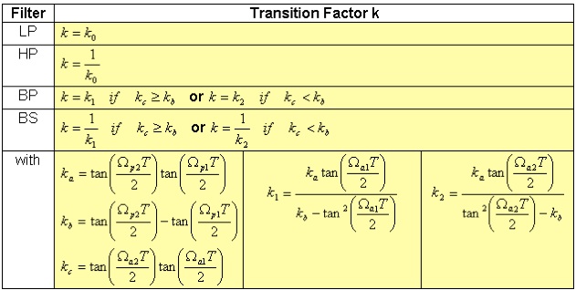
Table 3.6 Transition Factor for the Butterworth filters.

Regarding the above table, we indicated with k0 the inverse of the transition factor k. Ωa1 is the digital cutoff angular frequency of the first rejection band of a Bandpass filter, or the minimum angular frequency of the rejection band for a Bandstop filter.

Ωa2 is the lower cutoff angular frequency of the second rejection band of a Bandpass filter, or the higher cutoff angular frequency of the rejection band for a Bandstop filter. Similarly, Ωp1 and Ωp2 are the lower and higher cut off angular frequencies, respectively, of the pass band of a Bandpass filter, and the cutoff angular frequencies of the pass bands in case of Bandstop filter.

Considering the general transfer function H(s) formulae, at the beginning of this paragraph, for a Butterworth filter we need to perform the following replacements:

3.3.2 CHEBYSHEV FILTER

If the filter requirements are given, for instance, specifying the maximum approximation error in the pass band, a better approach could be to evenly spread the precision of the approximation in the pass band, or in the rejection band, or in both the bands.

To achieve this result, you can use the Chebyshev approximation for the attenuation function L. In this way, you obtain a constant ripple rather than a monotonic figure as for the previous filter. The filters that make use of such approximation have a frequency response module with a constant ripple behaviour in the pass band, and a monotonic behaviour in the rejection band (figure. 3.10.)

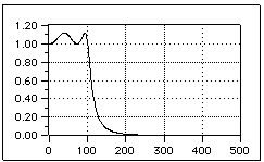
Fig. 3.10. Bode Diagram of the response module of a lowpass Chebyshev filter: with respect to the figure 3.9, here we used 3 poles instead of 6.

The main advantage of this type of filter, unlike the Butterworth ones, is that for the same filter design requirements, the filter order is lower (i.e. we need a lower n value). The normalised transfer function has the following form:

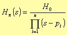
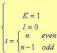
where the H0 constant value depends on n evenness:

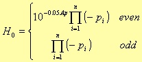
Once again, Ap is the pass band attenuation. In this case, the zeros of the lost function L lie on an ellipse circumscribed by the circumference of unitary radius [2].

A Chebyshev filter differs from the Butterworth one, also in the way the minimum number n of poles is computed. This is due to the different expression representing the attenuation.

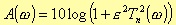
where

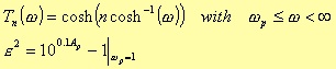
For  ω= ωa

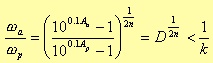
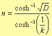
Where D, as for the Butterworth filter, is a power of the ratio ωa/ωp. In this way, it follows that

Therefore, for ωp = 1, the minimum value for n is

Nothing is formally changed for the transition factor k, so the table 3.7 is the same as the table 3.6.

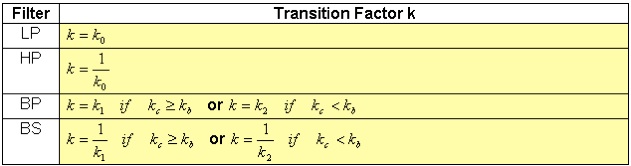
Table 3.7 Transition Factor for the Chebyshev filters: see also Table 3.6.

Considering the general transfer function H(s) formulae, at the beginning of this paragraph, for a Chebyshev filter we need to perform the following replacements:

3.3.3 ELLIPTIC FILTERS

The basic idea behind the elliptic filters comes considering that if you evenly spread the error over the whole pass band, as previously shown, than it is possible to match the filter design requirements with a lower filter order than when the error can grow monotonically (see Butterworth filter). Given these considerations, it is easy to think to evenly spread the error also over the rejection band. One way is the use an approximation coming from the elliptical function of Jacobi.

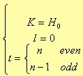
The normalised transfer function of the elliptical filter is more complex than the previous ones, and it has the following form

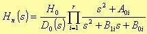
where r is (n-1)/2 when n is an odd number, and n/2 when even; D0(s) is s + s0 for the odd case, and 1 for the even one. Before considering the s0 value, we need to define the following parameters

where k is the transition factor, i.e. the ratio between the cutoff frequencies of the pass band and of the rejection one, in the case of a lowpass filter.

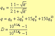
where Aa ed Ap are the attenuations in decibel of the rejection and pass band respectively. With these parameters, it is possible to calculate the minimum number of poles needed to match the filter design requirements.

We still need to introduce another parameter

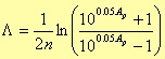
Finally

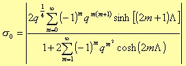
In order to represent the transfer function in more compact form, we need to define also

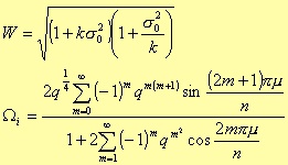
where the value of m is equal to i for odd values of n, and equal to i - ½ for even values of n. i goes from 1 to r.

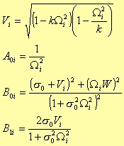
The transfer function is then

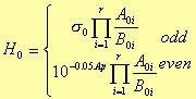
Figure 3.11 shows the Bode diagram of the impulse response module for an elliptical filter. (The design requirements are the same as for the previous cases.)

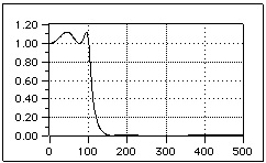
Fig. 3.11. Bode Diagram of the response module of a lowpass elliptical filter.

Considering the general transfer function H(s) formulae, at the beginning of this paragraph, for an elliptical filter we need to perform the following replacements:

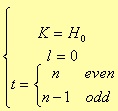
Table 3.8 shows how to transform the design of a lowpass for the others types: highpass, bandpass, and bandstop filters.

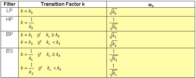
Table 3.8.

next >

< previous