In our instrument, the IIR filtering system is able to process one or more signals, up to 8, at the same time. Moreover, it is possible to select between three filter methods (Butterworth, Chebyshev, and Elliptic), using the typical filter configurations: lowpass, highpass, bandpass, and bandstop.

The input parameters are:

1. •the sampling frequency, which depends on the number of channels used (up to four per board) and from the number of acquisition boards (one or two).
   

2. •the attenuation in both the rejection and pass bands.
   

3. •the number of poles.
   

The setting of all these parameters can be done from a single front panel (see figure 3.13) in which you can also find a little display used to see the resulting filtered signal, and the Bode diagrams for the module and the phase of the selected filter.

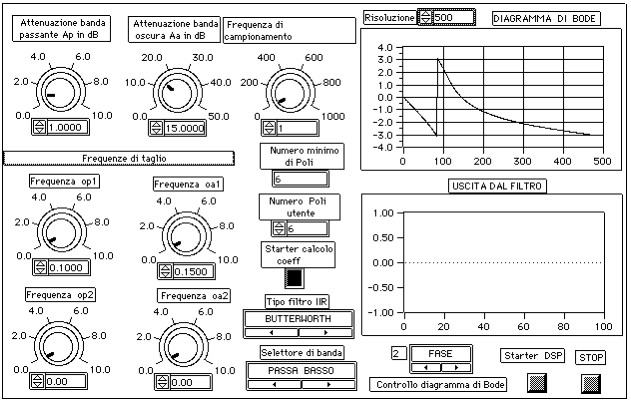
Fig. 3.13. Control Panel of the measurement instrument for the IIR filtering in Real Time. The labels are in Italian.

As you can see from figure 3.13, a set of “potentiometers” on the left side of the panel, let the user to input the attenuation bands in decibel, the sampling frequency in kHz, and the frequency range for the rejection and pass bands always in kHz. By two “switches”, the user can select the kind of filter and its approximation function method. By another “switch”, the user can set the number of poles. Further, it is possible to control in different phases the computation of the filter coefficients and the DSP processing start. In this way, once the coefficients computation has been completed, it is possible to modify and check the filter, via Bode diagrams, before proceeding with the signal processing.

The system is able to perform a sort of consistency checking for all of the parameters selected by the user. For instance, a wrong filter configuration could be obtained by selecting a lowpass filter with a pass band cut off frequency higher than the one of the rejection band. In such a case, the system warns the user with an error message describing the kind of error.

Finally, for each set of requirements input by the user, the system automatically suggests the minimum number of poles for the filter stability.

The first part of the algorithms, is located on the Host Computer: before proceeding with the acquisition and processing boards configuration, a set of sequences is needed to manage the different filter design phases. The first sequence consists of a Code Interface Node (CIN), which performs a check of all the parameters input from the front control panel. The second sequence consists of a CIN, in which the minimum number of poles is computed. A waiting sequence let the user to modify the parameters, and finally another CIN perform the coefficients computation; these coefficients are displayed by a specific CIN in the form of Bode diagram; it is at this point that the user may want to start the real time processing, or restart the filter design.

The code for all the sequences is placed in the “Pascal void CINRun” of the Code Interface Node. The same holds for the boards configuration CIN. Regarding the CIN for the data transfer to the DSP, we used:

1. •The CINInit to load the addresses of the variables “shared” between the Host Computer and the DSP.
   

2. •The CINDispose to handle the “end of job” flag.
   

3. •The CINRun to display the data.
   

Now it follows a description of the icon hierarchy used in LabVIEW, and the steps sequence of the IIR filter section of our instrument.

First, in the figure 3.14 we show the “iir” icon. This is the main icon we build for our instrument. This icon handles other two icons coming with LabVIEW: one icon regards the error handler for the values of the input parameters that are not compatible with the kind of selected measure (as for example, when selecting a sampling frequency lower than the signal period), and the other icon checks the real sampling frequency of the acquisition boards. In turn, these icons handle other icons: the one labeled “RATE” uses the icon “ID” (Identification Device) to know which is the unit to be polled; the other icon (Ask and Answer Dialog) handles the status register reading of the acquisition boards to retrieve information about the sampling frequency.

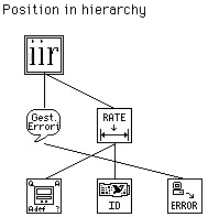
Fig. 3.14.

Figure 3.15 shows the first sequence of the measurement instrument, which handles the possible errors in the input parameters from the control panel. The central part, where different inputs from the control panel flow into, is the Code Interface Node (CIN).

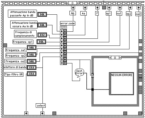
Fig. 3.15.

The second sequence (figure 3.16) calculates the minimum number of poles to match the user specifications.

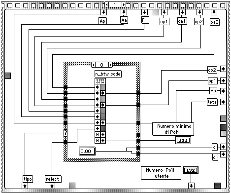
Fig. 3.16.

Next (figure 3.17), through a “switch” placed on the control panel, the user can start the sequence (figure 3.18) for the coefficients calculation, and therefore the Bode diagram sequence (figure 3.19).

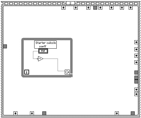
Fig. 3.17.

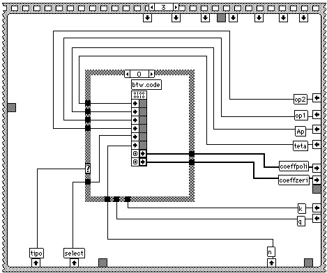
Fig. 3.18.

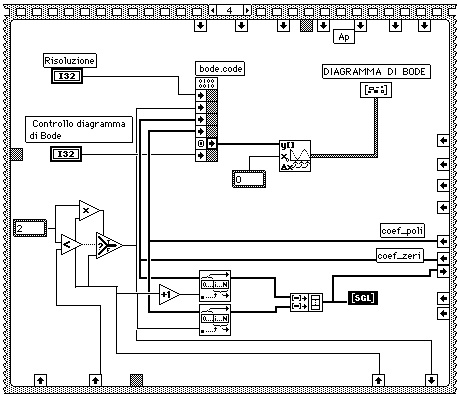
Fig. 3.19.

Another “switch”, always placed on the front panel, let the user to start the real time processing, once the Bode diagram shows a satisfactory filter response. After the sequence for this “switch” (figure 3.20), figures 3.21 and 3.22 show the sequence for the acquisition boards set up and the filtering sequence respectively.

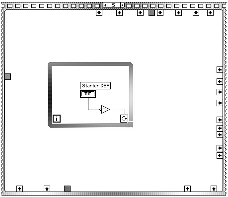
Fig. 3.20.

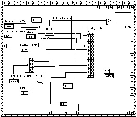
Fig. 3.21.

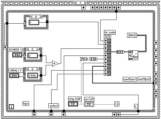
Fig. 3.22.

The code for the filtering and the real time processing is downloaded on the ONCHIP memory of the DSP. This code has been written in assembly, and it is made by four independent applications: a main program (Main), an interrupts handler, a filtering program, and last a program to convert data from the standard IEEE floating point format (used in the Host environment) to the Texas Instrument (TI) format, (used within the DSP), and vice versa.

All the pointers, to the different memory locations, are within the same memory space used by the executable code: in this way, we prevented the system from performing several and unnecessary page commutations. The variables used to store the addresses passed by LabVIEW, have been placed in the Dual Access memory, because this is the only memory the Host can access directly without the use of interrupts. The filter coefficients, read by the DSP from the Mac, are first loaded from the Host Computer memory into the DSP Dual Access memory. Then, before the real time processing, it is up to the Main program, to move these coefficients directly into the ONCHIP memory (the average number of the coefficients is not very high, and generally much lower than a hundred).

However, the tasks performed by the Main program can be briefly described through the following points:

1. 1.It disables the interrupts number 1 and 2 of the RTSI bus and the DMA respectively.
   

2. 2.It loads the user parameters from LabVIEW (at this point LabVIEW has already passed the addresses to the DSP). Read the needed parameters (as the selected number of acquisition channels or the number of point on which the filtering is going to be performed) and store the information in the Dual Access memory.
   

3. 3.It initialises the pointers to the proper buffers, depending on the number of working channels, and downloads the filter coefficients. Change the coefficients format from IEEE to TI floating point representation and place the data ONCHIP.
   

4. 4.It initialises the variables used to start the IIR filter routine. At this point, the reading of the LabVIEW parameters is completed and the Main set the proper status flag on the Host.
   

5. 5.It loads the interrupt vector #1.
   

6. 6.It configures the DSP Control Register and clears all the data buffers.
   

7. 7.It sets the internal timer, and initialises the pointers to access the two acquisition boards. It loads the address of the Soft A/D Clear Strobe Register in order to be able to clear the FIFO buffers when necessary.
   

8. 8.It enables the interrupt #1 for the data acquisition because now the sampling is started, and the real time processing can take place.
   

9. 9.It starts the “wait” loop for the data processing and the data transfer to the Macintosh host: first, the Main is in the IDLE state, waiting for the interrupts. When the interrupt occurs, the Main checks whether the “end of job” or the “parameters change” flags have been changed or not under LabVIEW. In case the “end of job” flag is set, the Main jump at the end of the program (step 13). In case the “parameters change” flag is set, the Main jump at the beginning (step 1) of the program where it disables the interrupts, and loads again the new parameters.
   

10. 10.After the flag control, the Main checks how many interrupts occurred to see if there are enough data to start the signal processing. For instance, in case of 4 acquisition channels, for each acquisition interrupt, there are 512 data available per board in the DSP Dual Ported memory (i.e. 256 samples for channel.) In order to filter 1024 samples, the Main waits for 4 interrupts.
    

11. 11.Once there are enough data, the filtering nested loops are executed for each channel.
    

12. 12.At the end of the processing, data are transformed back to the IEEE floating point format, the one used in the Macintosh environment, and transferred to LabVIEW to can be displayed. The code jumps back (step 9), at the beginning of the “wait” loop.
    

13. 13.This last step is executed when the Main find the “end of job” flag has been set. Before enter into the IDLE state, the DSP enables again the interrupts. In this way, the Host Computer is free to download new software. From here, the DSP is not longer the Master of the communication, and it waits for new instructions.
    

The tasks for the interrupt handler are:

1. 1.To store all the DSP register into the stack.
   

2. 2.To configure the DMA Controller for a block data transfer from the acquisition boards to the DSP Dual Ported memory. The input samples are packed: each transferred word contains two words of sampled data.
   

3. 3.To check by polling, if the data transfer from the boards is completed.
   

4. 4.To configure the DMA data transfer from the second acquisition board, once the DMA data transfer from the first board is finished.
   

5. 5.To unpack the samples from the first board into the Dual Access memory, so that the DSP can start to process them (while the samples from the second board are coming via NuBus.)
   

6. 6.To check if the DMA Controller has finished to transfer the data from the second board.
   

7. 7.To unpack the samples from the second board into the Dual Access memory, so that the DSP can start to process them.
   

8. 8.To restore the DSP registers
   

9. 9.To return to the Main.
   

The procedures for the data unpacking and for the data transfer have to know the number of channels actually in use, in order to properly store the data into the Dual Access memory.

Figure 3.23 shows the three adjacent 512-word memory locations, which hold the input signal samples coming from one channel. The interrupt routine stores the samples filling up the three buffers in a cyclic way.

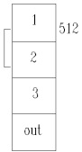
Fig. 3.23. A Buffer in Dual Access memory to store the samples and the data results.

The table 3.9 shows the experimental results obtained at the maximum sampling frequencies to process in real time data coming from two up to eight channels at the same time.

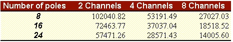
Table 3.9. Frequencies in Hz.

The DSP check if there are enough data to proceed with the processing, every 2870ns. This time interval is necessary to guarantee that no overflow will occur in the acquisition boards. In fact, we could set other time values, but we had data overflow on the acquisition boards. The value 2870 comes after a time evaluation we did on the processing time required by the DSP. Then, this time interval has been verified run time.

Indeed, the optimal time interval depends on both the number of channels used, and on the filter poles number. In our design, we preferred to optimise the configuration where there are two channels only, and an high number of poles: about the other configurations left, we observed lower values of the maximum sampling frequencies, with differences from zero to 3kHz, than the selected configuration case. In fact, the maximum sampling frequencies distribution as a function of the polling time intervals shows a flat local maximum for intervals less than the evaluated one and it decreases quicker for greater intervals than our 2870ns.

next >

< previous